Geoscience Reference
In-Depth Information
Exponential scheme
As discussed in Section 4.2.1.2, if
ρ
u
and
are assumed to be constant, Eq. (4.103)
has an exact solution. If a domain 0
≤
x
≤
L
is considered, with boundary conditions
φ
=
φ
0
at
x
=
0 and
φ
=
φ
L
at
x
=
L
, the solution of Eq. (4.103) is
φ
−
φ
exp
(ρ
ux
/)
−
1
0
0
=
(4.115)
φ
−
φ
exp
(ρ
uL
/)
−
1
L
dx
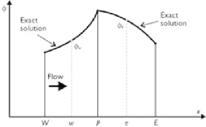
. Using the exact solution (4.115) as a profie
between points
P
and
E
, as shown in Fig. 4.17, yields the expression for
I
w
:
Define the total flux
I
=
ρ
u
φ
−
d
φ/
F
w
+
φ
−
φ
W
P
I
w
=
φ
(4.116)
W
exp
(
P
w
)
−
1
Substituting Eq. (4.116) and a similar expression for
I
e
into Eq. (4.104) leads to
F
e
F
w
φ
−
φ
+
φ
−
φ
P
E
W
P
φ
+
−
φ
=
0
(4.117)
P
W
exp
(
P
e
)
−
1
exp
(
P
w
)
−
1
which can be written as Eq. (4.108) with coefficients:
F
w
exp
(
F
w
/
D
w
)
a
W
=
exp
(
F
w
/
D
w
)
−
1
F
e
a
E
=
(4.118)
exp
(
F
e
/
D
e
)
−
1
a
P
=
a
W
+
a
E
+
(
F
e
−
F
w
)
The exponential scheme (4.117) is based on the formulation first presented by
Spalding (1972). It is similar to the exponential difference scheme introduced in
Section 4.2.1.2.
Figure 4.17
Sketch of exponential scheme.