Geoscience Reference
In-Depth Information
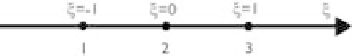
Figure 4.12
1-D local element.
1
2
T
{
(
2
e
P
ξ
−
e
−
P
e
P
c
1
=
−
)
+
T
[
1
−
ξ(
R
+
1
)
]}
1
2
T
{
(
2
e
P
ξ
−
e
−
P
e
P
c
3
=
−
)
+
T
[
1
−
ξ(
R
−
1
)
]}
(4.100)
c
2
=
1
−
c
1
−
c
3
e
−
P
e
P
e
P
e
−
P
where
T
=
+
−
2,
R
=
(
−
)/
T
,
P
is the Peclet number defined as
P
=ˆ
u
/ε
ξ
,
u
is the local velocity, and
ε
ξ
is the diffusion coefficient.
Fig. 4.13 shows the behavior of the upwind interpolation functions at various Peclet
numbers. It can be seen that these functions become more asymmetric as the Peclet
number increases, i.e., when convection becomes more dominant. This upwind feature
stabilizes this interpolation method in the simulation of strong convection problems.
The upwind interpolation functions in 2-D and 3-D cases can be obtained by apply-
ing Eq. (4.100) in every direction. For example, the upwind interpolation functions
for the 2-D element shown in Fig. 4.8 are constructed by
ˆ
ϕ
k
=
c
i
(ξ)
c
j
(η)
(4.101)
where
k
is corresponding to the pair of
i
and
j
according to Table 4.1.
Figure 4.13
Upwind interpolation functions.
This upwind interpolation method is called the efficient element method by Wang
and Hu (1993). It has been used in hydrodynamic modeling by Jia and Wang (1999).