Geology Reference
In-Depth Information
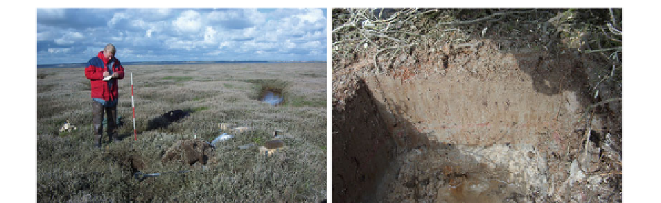
Fig. 8.16
Excavation of one of the test sides on the salt marsh of
the Skallingen backbarrier. The location at the time of excavation in
2003 is shown to the
left
. To the right is seen the excavated trench
with about 20 cm salt marsh clay (
brown
) above the sand base (
light
grey
). A few cm
above
the old sand surface there is a
red-collared
horizon. This is the marker horizon consisting of
red-collared
sand
spread on the salt marsh surface by Nielsen in the 1930s (Nielsen
1935
) (Photos courtesy of Jørn Bjarke Torp Pedersen)
area per year which, by division with the bulk dry
density of newly deposited material, gives D
S
sed
. This
procedure has been programmed with various editions
of Eqs.
8.7
and
8.8
by Temmerman et al. (
1993
) who
also incorporated a mathematical description of the
tidal curve and by French (2006), who incorporated
the compaction term described in Eq.
8.1
.
The basic assumptions by means of which this
model is implemented provide limitations. Perhaps
the most important of these is the assumption of a
constant value of
C
0
, as it is clear from observations
(Fig.
8.3
) that
C
0
is not constant over the tidal period.
Temmerman et al. (
2003
) allow
C
0
to vary as a linear
function of the high tide level (but keep it constant
over the tidal period), whilst French (2006) considers
it to be constant for and during all modelled tidal peri-
ods. Both regard the settling velocity,
w
s
, to be con-
stant, even if it undoubtedly decreases with time
during a tidal period, and most likely in general fol-
lows an expected variation in
C
0
. Being in the open,
these limitations do not disqualify the two models, but
contribute to classify them as fi rst approximations
based on which more work should be done to improve
their performance.
Bartholdy et al. (
2004,
2010a
) used another
approach. Their database allowed them to evaluate
accurate accretion measurements in three lines across
the Skallingen backbarrier (Fig.
8.1
) over a period of
more than 60 years. This database was founded by
Nielsen (
1935
) who spread out red-coloured sand on
the surface of what then was a juvenile backbarrier salt
marsh. The marker horizon can be seen in an exca-
vated trench dug in 2003 (Fig.
8.16
).
This model assumes that in time, the average depo-
sition (kg m
−2
tidal period
−1
) at a specifi c site, related to
a specifi c high water level (
HWL
), is equivalent to:
[
]
Δ=Δ
s
C
L
−
E t
()
(8.11)
sed
(HWL)
where
E
(
t
) is the salt marsh elevation at the specifi c
location and D
C
(HWL)
is the characteristic concentration
difference available for deposition. D
C
(HWL)
is regarded
as place specifi c but dependent on the high water level
relative to the mean high water level (
MHWL
):
(
)
Δ
C
=
α
ln
HWL
−
MHWL
+
β
; valid for HWL
>
MHWL
(8.12)
(HWL)
The mean high water level is supposed to be
the level of salt marsh initiation. The model was
formulated in a Fortran program where all high water
levels were grouped in classes of 0.2 m steps above
the mean high water level and assigned the class
midpoint as its level. Observations in the salt marsh