Hardware Reference
In-Depth Information
servers at 10% utilizations, etc. Compute the total performance and total energy for
this workload mix using the assumptions in part (a) and part (b).
d. [20] One could potentially design a system that has a sublinear power versus load
relationship in the region of load levels between 0% and 50%. This would have an
energy-efficiency curve that peaks at lower utilizations (at the expense of higher utiliz-
ations). Create a new version of column 3 from
Figure 6.4
that shows such an energy-
eiciency curve. Assume the system utilization mix in column 7 of
Figure 6.4
.
For sim-
plicity, assume a discrete distribution across 1000 servers, with 109 servers at 0% util-
ization, 80 servers at 10% utilizations, etc. Compute the total performance and total
energy for this workload mix.
6.30 [15/20/20] <6.2, 6.6> This exercise illustrates the interactions of energy proportionality
models with optimizations such as server consolidation and energy-efficient server
designs. Consider the scenarios shown in
Figure 6.26
and
Figure 6.27
.
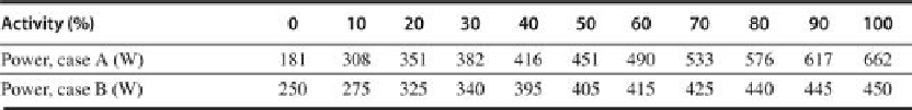
a. [15] Consider two servers with the power distributions shown in
Figure 6.26
: case A
(the server considered in
Figure 6.4
) and case B (a less energy-proportional but more
energy-eicient server than case A). Assume the system utilization mix in column 7
of
Figure 6.4
.
For simplicity, assume a discrete distribution across 1000 servers, with
109 servers at 0% utilization, 80 servers at 10% utilizations, etc., as shown in row 1 of
Figure 6.27
. Assume performance variation based on column 2 of
Figure 6.4
.
Compare
the total performance and total energy for this workload mix for the two server types.
b. [20] Consider a cluster of 1000 servers with data similar to the data shown in
Figure
6.4
(and summarized in the first rows of
Figures 6.26
and
6.27
)
. What are the total
performance and total energy for the workload mix with these assumptions? Now as-
sume that we were able to consolidate the workloads to model the distribution shown
in case C (second row of
Figure 6.27
). What are the total performance and total energy
now? How does the total energy compare with a system that has a linear energy-pro-
portional model with idle power of zero wats and peak power of 662 wats?
c. [20] Repeat part (b), but with the power model of server B, and compare with the res-
ults of part (a).
FIGURE 6.26
Power distribution for two servers
.
Search WWH ::

Custom Search