Image Processing Reference
In-Depth Information
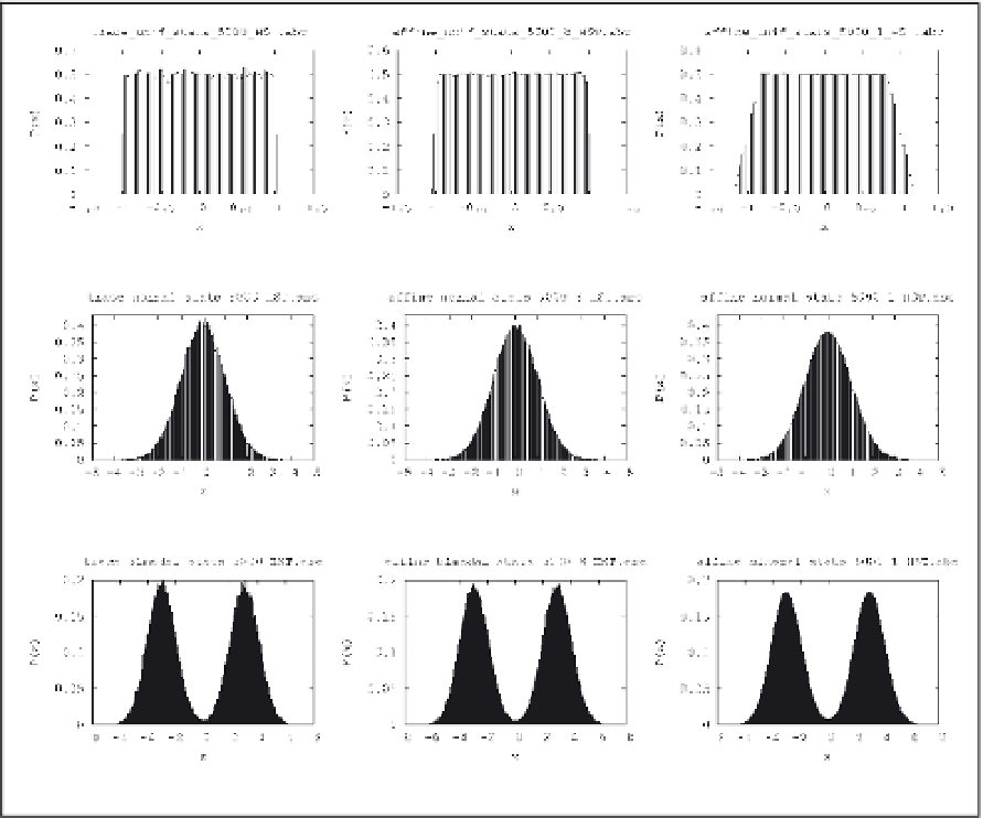
whose width is set to the variance of the distribution. All the histograms have been
computed using 20 averages of 5000 data items each. It can be seen that the areas near the
edges on the uniform distribution are modified, but the remaining parts of the distribution
are also computed taking into account a larger number of points. It is also noticeable that the
new PDFs are smoother than the ones computed using the numerical traces, which can be
explained from the Central Limit Theorem.
(a) (b) (c)
(d) (e) (f)
(g) (h) (i)
Fig. 6. Distributions generated using traces of numbers, traces of intervals whose widths are
set to 1/8 of the variance, and traces of intervals whose widths are set to the variance of the
distribution. These traces are applied using the Monte Carlo Method to: (a) - (c) a uniform
distribution in [-1, 1]; (d) - (f) a normal distribution with mean 0 and variance 1; (g) - (i) a
bimodal distribution with modes 3 and -3 and variance 1.
Figure 7 details the central part and the tails of a normal distribution generated using traces
of 100000 numbers and 5000 intervals. It can be observed that the transitions of the
histograms are much smoother in the distribution generated using intervals. Although there
are slight deviations from the theoretical values, these deviations (approximately 5% in the
central part and 15% in the tails) are comparable to the deviations obtained by the numerical
trace using 100000 numbers.