Image Processing Reference
In-Depth Information
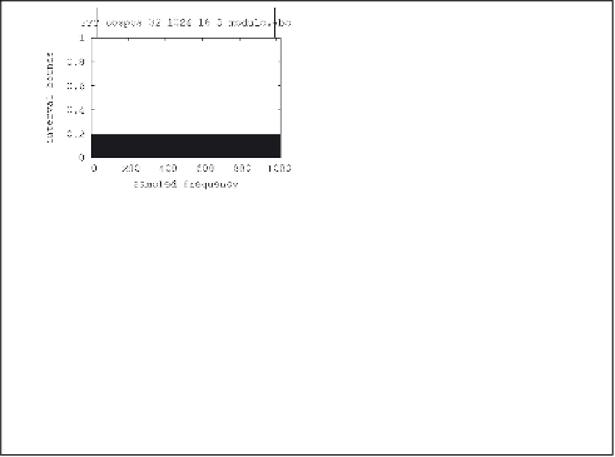
(a) (b)
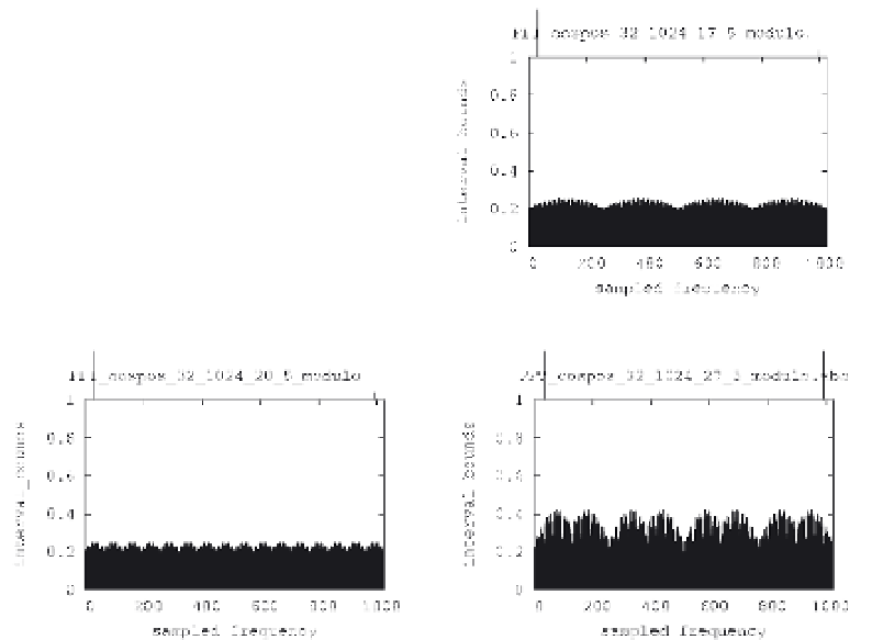
(c) (d)
Fig. 5. Details of the ripples that occur in the transformed domain due to the presence of
uncertainty intervals in the deterministic signals: (a) in a position which is a factor of the
number of FFT points (16). (b) - (d) in other non-factor positions (17, 20 and 27, respectively).
The vertical lines above the figures indicate the positions of the deltas, whose heights exceed
the representable values in the graph.
The first part of this section analyzes the changes in the PDFs. To do this, data sequences
following a particular PDF are generated, and they are later reconstructed and compared
with the original results. The steps used to perform the experiments are as follows:
1.
Generate the traces of the random samples following the specified PDF, and assign the
width of the intervals.
2.
Obtain the histogram of the trace, group the samples and plot the computed PDF.
3.
Repeat steps 1 and 2 to reduce the variance of the parameters (
M
times).
4.
Average the histograms obtained in step 3.
5.
Repeat the previous steps assigning other interval widths.
Step 1 generates the sequences of samples that follow the specified PDF, and in step 2 the
PDFs are recomputed from these samples. In this experiment, three types of PDFs have been
used: (i) a uniform PDF in [-1, 1], a normalized normal PDF (mean 0 and variance 1), and a
bimodal PDF composed of two normal PDFs, with means -3 and 3 and variance 1. Steps 3
and 4 have been included to reduce the variance of the results. Finally, step 5 allows
selecting other interval widths.
Figure 6 presents the results of the three histograms using the Monte-Carlo method with: (i)
numerical samples, (ii) intervals whose width is set to 1/8 of the variance, and (iii) intervals