Image Processing Reference
In-Depth Information
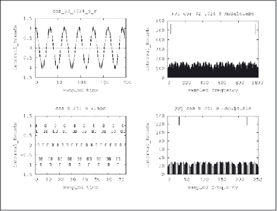
shows another cosine signal of the same amplitude and width, length 256 and period 8.
Figures 3.b and 3.d show the computed FFTs for each case, where each black line
represents a data interval.
(a) (b)
(c) (d)
Fig. 3. Examples of FFTs of deterministic interval signals: (a) First 200 samples of a cosine
signal of length 1024, period 32, and interval widths 1/8 in all the samples. (b) FFT of the
previous signal. (c) First 75 samples of a cosine signal of length 256, period 8, and interval
widths 1/8 in all the samples. (d) FFT of the previous signal.
As expected, these figures clearly show that the output intervals in the transformed domain
have the form of the numerical transform, plus a given level of uncertainty in all the
samples. In addition, Figures 3.b and 3.d also provide: (i) the values of the deviations in the
transformed domain in each sample with respect to the numerical case, and (ii) the
maximum levels of uncertainty associated with the uncertainties of the inputs.
The second part of this experiment evaluates how each uncertainty separately affects to the
FFT samples. As mentioned above, by performing a separate analysis of how each
uncertainty affects to the input samples, we are characterizing the quantization effects of the
FFT. In this case, step 3 is replaced by the following statement:
3. Include one uncertainty in the specified sample of the input signals.
which is performed by generating a delta interval in the specified position, and adding it to
the input signal.