Image Processing Reference
In-Depth Information
and un-weighted residuals are zero. Finding the
K
sinusoids that solve eq. (8) is the
standard NLS problem and if this were computationally tractable, the problem would be
solved. But as pointed out by Li et al. (2000) [see also the discussion in Stoica & Moses
(1997)], “the NLS cost function in (3) is usually multimodal with many local minima,” and
“the minimization of the NLS cost function requires the use of a very fine searching
algorithm and may be computationally prohibitive.”
One way out of this dilemma is to use NLS in place of least squares within OMP. This has
two advantages over using NLS by itself. First, the frequency band over which one has to
search in NLS is reduced from the entire frequency band to the frequency grid spacing in
the over-complete dictionary used in OMP. Second, the estimates of the frequencies at any
given iteration are improved from the values on the grid by using NLS in the previous
iteration (see the discussion of a similar continuous version of matching pursuit by Jacques
& De Vleeschouwer, 2008).
The first step in our formulation is to define the vector function of frequency,
x
(
f
), as the
time series for a unity amplitude complex sinusoid at frequency
f
evaluated at integral
sampling times
t
= 0 to
t
=
N
-
1,
x
(
f
) = [1, e
i2π
f
, e
i4π
f
, ... , e
i2(
N-
1)π
f
]. (9)
Note that the solution for
X
S
in eq. (5) is a linear combination of
K
vectors
x
(
f
i
), (
i
= 1,
K
). To
use OMP, we need an over-complete dictionary (Candes et al., 2010) which means that
x
(
f
)
is evaluated on a fine grid oversampled by the factor
N
f
from the DFT grid. The second step
is to define a function that can be evaluated on the fine grid to find a grid frequency close to
one of the true frequencies in the input signal
X
s
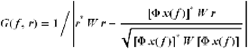
. Here we use the function
G
(
f
,
r
) given by
(10)
where initially
r
=
y
and subsequently,
r
equals the residual of
y
with 1 to
K
components
removed as discussed below. We calculate the argmax of
G
(
f
,
y
)
over
f
in the dictionary
frequencies to make a first estimate of one of the frequencies present in the input signal
X
(
t
).
If there is no noise and if there is only one sinusoid, this procedure provides the dictionary
vector whose frequency is nearest that of the input sinusoid. If multiple sinusoids are
present, the maximum of
G
(
f
,
y
) occurs at one of the dictionary vectors whose frequency is
near one of the input sinusoids provided that the dictionary is sufficiently over-complete
and that
Φ
possesses the restricted isometry property (Duarte and Baraniuk, 2010). Note
that
G
(
f
,
r
) is the inverse square of the distance between
r
and the linear span of
x
(
f
)
in the
W
-normed inner product space (defined by <
a
,
b
> =
a
H
Wb
). Thus finding the argmax of
G
(
f
,
r
)
is equivalent to finding the argmax of the inner product of the residual with the
product of
Φ
times the dictionary vectors
x
(
f
j
)
for all
f
j
on the over-complete frequency grid
(see Tropp and Gilbert, 2007, Algorithm 3, Step 2).
Given estimates of the frequencies
{
f
1
,
f
2
,…
f
K
}
present in the input signal, we can find
estimates of the amplitudes of each sinusoid by using the least squares estimator
A
(
U
)
for
the amplitude vector
{
a
1
,
a
2
,…
a
K
}
(see Stoica and Moses, 1997, eq. 4.3.8 and Stoica et al., 2000)
A
(
U
) = (
U
H
W U
)
-1
U
H
W y
(11)