Image Processing Reference
In-Depth Information
Finally, amplitude and phase responses are showed on Eq. 6 and Eq. 7, respectively.
sen
2
H
()
(6)
sen
2
(7)
()
(
1)
2
The filter's group delay is
(
, and the associated gain for ω=0 is α determined
)
2
evaluating |H (ω=0)|.
Once completely characterized the low-pass filter, designing the high-pass filter is an easy
task using the following transfer function:
(
)
(
)
1
(
)
1
z
1 /
z
2
z
2
z
/
Hz
()
z
2
/
(8)
1
1
1
z
1
z
This filter can be implemented directly by the following difference equation:
(
)
(
)
yn
[]
yn
[
1]
xn
[]/
x n
x n
1
xn
[
]/
(9)
2
2
Getting amplitude response for this filter is mathematically complex. Nevertheless,
theoretically this filter must have the same cut frequency of the subjacent low-pass filter in
inverse order. Furthermore, the values of phase response and group delay of the high-pass
filter are the equal to the same parameters for the low-pass filter (Smith, 1999).
For a cut frequency of 430 Hz, α values and associated cut frequency (-3 dB.) are shown on
Table 3.
Valor de α
Frecuencia de Corte
850
0.2 Hz.
320
0.5 Hz.
35
5 Hz.
Table 3. Cut Frequencies of High-Pass Lynn Filter
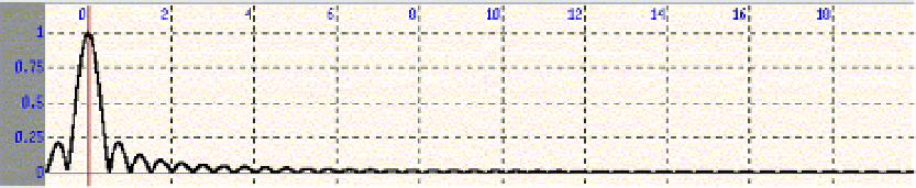
Figures 14, 15 and 16 show the low-pass filter amplitude response which give an idea of the
amplitude response of the associated high-pass filter because the cut frequencies are the same.
Fig. 14. Low-Pass / High-Pass Lynn's Filter Amplitude Response - Cut Frequency 0.2 Hz