Environmental Engineering Reference
In-Depth Information
a very simple manner, but also provide useful design guidelines by
highlighting the properties and limitations implicit in specific types of
feedback configurations.
3.2 SIGNAL FLOW GRAPH ANALYSIS
Classical SFG techniques have never gained popularity not only in circuit
design but even for analysis. This is mainly due to uncertainties in
transcribing circuit diagrams into their SFG equivalents. Mason himself
recognized that the construction of a SFG is somewhat obscure, and that “A
link in the chain of dependency is limited in extent only by one's perception
of the problem.” Although some of these drawbacks have been overcome
[K00], the method still remains less direct than those proposed by
Rosenstark and Choma, which will be the only one comprehensively
considered in this text and described in the following sections. However,
since these methods descend from SFG through which they can easily be
demonstrated, we need to introduce some elementary concepts of SFG
analysis.
A signal flow graph allows us to graphically represent a circuit (or more
generally, a system) through the links between system variables. The nodes
on the graph represent variables and the relations among them consist in the
branches between the nodes with their associated weights. As a result, a
variable is the linear superposition of the node variables at the source of
incoming branches.
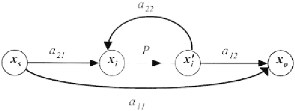
A general linear circuit can be represented by the signal flow graph
shown in Fig. 3.2. Variables and represent the input and output signals,
moreover, two other generic variables, and linked together through the
control (or
critical
) parameter
P,
are explicitly shown. Parameters are the
weight branches. Variables and the control parameter,
P,
can model a
controlled generator, or the relation between voltage and current across two
nodes of the circuit. This representation is particularly suited to feedback
circuits.