Geoscience Reference
In-Depth Information
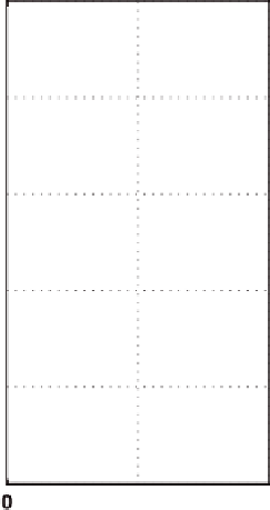
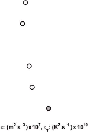
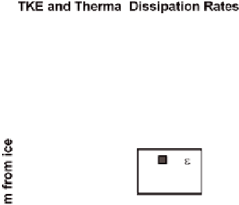
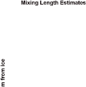
Fig. 5.2 a
TKE and thermal variance dissipation rates versus depth at ISW 92.
b
Estimates of
mixing length derived from spectral peaks
(
λ
peak
)
, from the TKE balance assuming production
equals dissipation
(
λ
ε
)
, and from the thermal variance conservation equation
(
λ
T
)
(Adapted from
McPhee and Martinson 1994. With permission American Association for the Advancement of
Science)
where
u
∗
is the
local
friction velocity. This differs from the similarity model dis-
cussedinChapter4inthat
K
isallowedtovaryin theouterlayer,while weassume
that
remainsrelativelyconstant.
Without resorting to similarity scaling or mixing-length arguments, it is possi-
ble to estimate a representative eddy viscosity during the ISW storm directly from
Ekman theory. If the kinematic stress magnitude is exponential, i.e.,
λ
τ
=
τ
0
e
az
,we
can estimate the parameters
τ
0
and
a
by the linear regression of log
τ
versus
z
.Re-
sults ofthefittingareshowninFig.5.3.FromtheEkmansolution
2
a
2
K
fit
=
f
/
(
)
026m
2
s
−
1
.
The ratheruniquedataset fromtheISW storm also providesa credibleestimate
ofthescalar thermaleddydiffusivityaveragedthroughtheentireIOBL,byrelating
directly the vertical averaged kinematic heat flux
where
a
istheslopeofthesemilogarithmicfit.With
a
=
0
.
051
,
K
fit
=
0
.
and thermal gradient.
With an average heat flux of less than 10Wm
−
2
during the ISW storm, a rough
estimate of the expected thermal gradient in the well mixed layer may be made by
assumingthateddyscalardiffusivityiscomparabletoeddyviscosity
(
w
T
)
02m
2
s
−
1
(
0
.
)
: