Graphics Reference
In-Depth Information
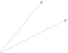
Fig. 11.13
Spherical
interpolation between
q
1
and
q
2
One of the reasons for using this spherical interpolant is that it linearly inter-
polates the angle between the two quaternions, which creates a constant-angular
velocity between the quaternions. However, one of the problems with visualising
quaternions is that they reside in a four-dimensional space and create a hyper-sphere
with a radius equal to the quaternion's magnitude. With our 3D brains, this is diffi-
cult to visualise. Nevertheless, we can convince ourselves into thinking we see what
is going on with a simple sketch, as shown in Fig.
11.13
, where we see part of the
hyper-sphere and two quaternions
q
1
and
q
2
. In this example, the angle
φ
is a con-
stant angle between two values of the interpolant
t
. The spherical interpolant also
ensures that the magnitude of the interpolated quaternion remains constant at unity
and prevents any unwanted scaling.
Figure
11.14
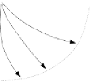
provides another sketch to help visualise what is going on. For ex-
ample, when
t
0, the interpolated quaternion is
q
1
which rotates the point
(
0
,
1
,
1
)
to
(
1
,
1
,
0
)
, and when
t
=
=
1, the interpolated quaternion is
q
2
which rotates the point
(
0
,
1
,
1
)
to
(
0
,
0
.
5, the interpolated quaternion rotates the point
(
0
,
1
,
1
)
to
(
1
,
0
,
1
)
as computed above. Two other curves show what happens for
t
−
1
,
1
)
. When
t
=
0
.
75.
A natural consequence of the interpolant is that the angle of rotation is 90° for
t
=
=
0
.
25 and
t
=
0
.
5 the angle of rotation (eigenvalue) is approximately
70
.
5°. Corresponding angles arise for other values of
t
.
0 and
t
=
1, but for
t
=
Fig. 11.14
Sketch showing
the actions of the interpolated
quaternions