Emitter Based Algorithm for Pressure-Driven Demand Calculations of Water Distribution Networks - Pattern Recognition for Reliability Assessment of Water Distribution Networks - page 39

1

( ) n

1

3.6

Q = H − z

i i i

1 n

K

i

Strictly speaking, the K -value in Equation 3.6 stands for the resistance of the dummy pipe,
but actually it has the same meaning as in Equations 3.2 to 3.4. Finally,

α

 p  p 1

Q = k 



i




;

i

= H − z ; α = 1 n ; k = 3.7

i i i i i α

ρ g ρ g K

i

where k i stands for the emitter coefficient in node i and α is general emitter exponent.

Emitter coefficients were first introduced in EPANET to simulate operation of fire hydrants.
By specifying the emitter coefficient, the demand node would turn into an emitter node. In
essence, this is a node in which the demand shall be adjusted based on the actual pressure in
the system, following Equation 3.7. The default value for exponent α in EPANET is 0.5,
which can be adjusted if necessary. Using the emitter approach gives clear advantages while
exploring the effects of pressure management on the leakage reduction in the system.
Furthermore, by connecting an emitter node to the normal consumption node (with a dummy
pipe of low resistance), the amount of water loss shall be clearly visible, although the size of
the model increases significantly. In the analyses of failures, EPANET has to be upgraded
with the value of pressure threshold which will be used to switch between the DD- and PDD
mode of calculation. Turning the DD hydraulic calculations into a PDD mode, the nodal
demands being an input in the DD mode then become dependent on the nodal pressure that is
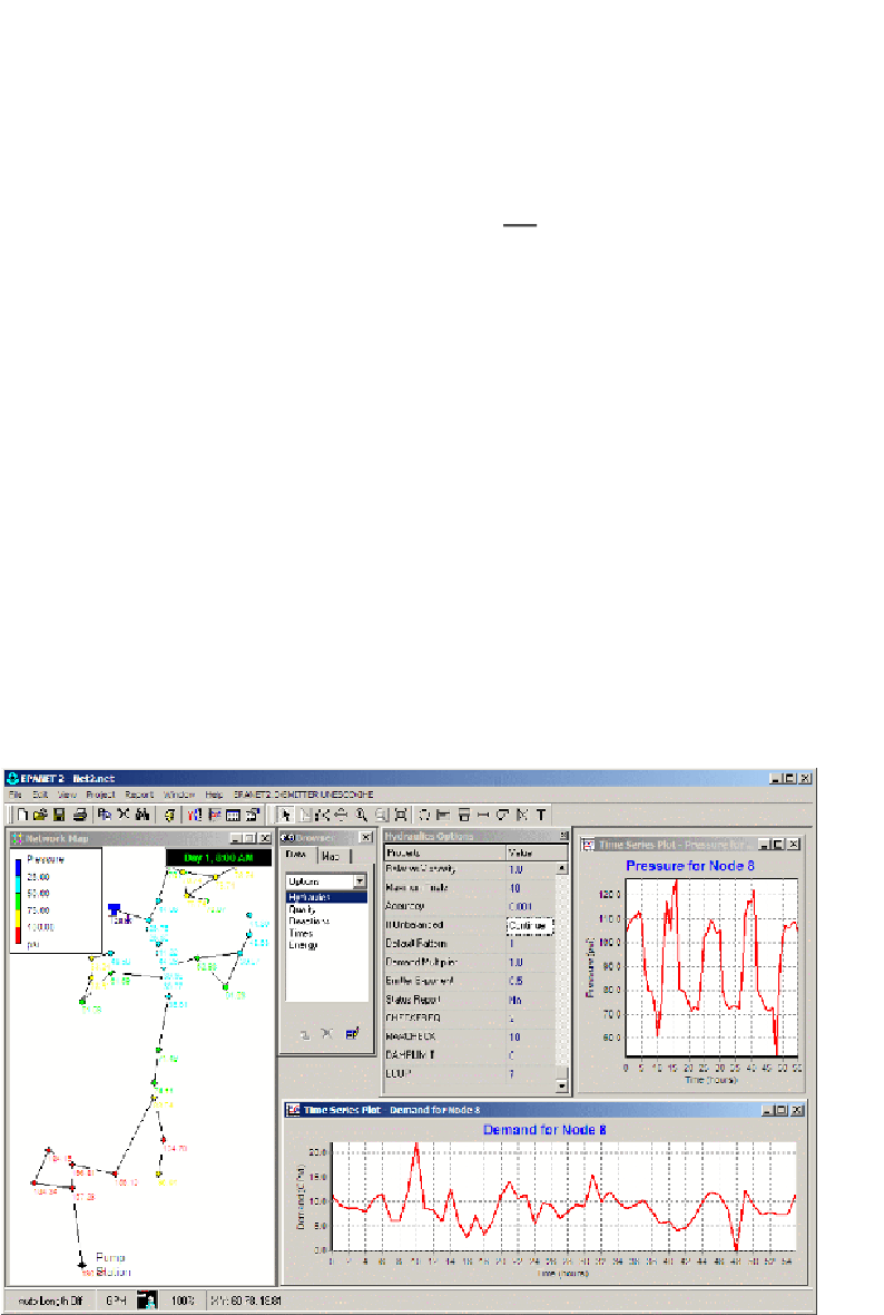
an output parameter, as long its value is below the threshold value. A PDD add-on has been
developed by Pathirana (2010) who defines an emitter cut-off point ( ECUP ) which is the
PDD threshold pressure.

Figure 3.5 User specification of PDD threshold pressure (ECUP) in EPANET (Pathirana, 2010)