Diagnostics of Regular Performance of Water Distribution Networks and its Relation to the Network Reliability - Pattern Recognition for Reliability Assessment of Water Distribution Networks - page 193

results in Tables 7.4 and 7.5 could be more meaningful, because the link between these two
parameters is not direct. Thus, in case each of these two parameters shows consistently good
correlation with the loss of demand, their mutual good or bad correlation could suggest the
level of demand loss even without running pipe failure analyses.
The results in Table 7.5 do not entirely come as a surprise knowing that GA-optimised looped
networks transform into 'quasi-branched' layouts, which was elaborated in Chapter 5. In
perfectly designed branched network, the relation between the pipe flow and volume
becomes clearer. This can be seen in the simple example shown in Figures 7.15 and 7.16, and
Table 7.13.
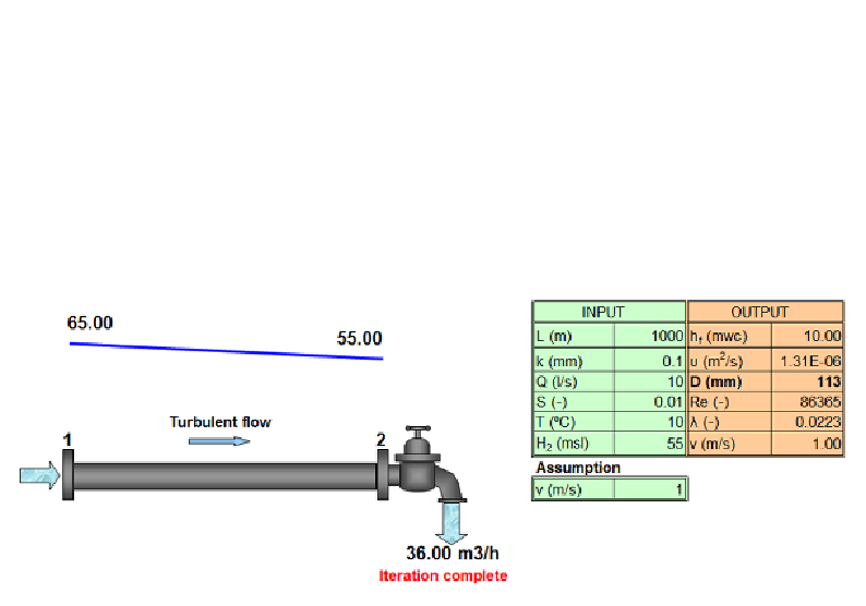
Figure 7.15 Calculation of pipe diameter at fixed value of flow and hydraulic gradient (Trifunović, 2006)
A single pipe of fixed length and roughness value can be optimised for fixed value of
hydraulic gradient and the range of flows. It is a simple iterative process that can be easily
conducted in a spreadsheet like the one in Figure 7.15 (Trifunović, 2006). The results for the
pipe shown in the figure, and the range of flows between 10 and 150 l/s at fixed value of
hydraulic gradient of S = 0.01, give the range of diameters between 113 and 315 mm,
respectively, as can shown in Table 7.13. The corresponding volumes are calculated for the
pipe length of 1000 m and the roughness value k = 0.1 mm. The correlation between the
flows and diameters/volumes is obvious. The Pearson's correlation between the values of Q
and V yields the coefficient 0.997 leading to a perfect exponential curve shown in Figure
7.16. For selected units, V = 0.0018 Q 0.7562 .
Assuming that this pipe belongs to a serial or branched network, its failure would mean the
loss of demand equal to its flow under regular conditions. Consequently, for selected
distribution of demands, and selected source head and minimum pressure in the network, the
diameter of each pipe can also be calculated for the known flow and the friction loss value;
thus, each demand scenario will have its optimal network. Eventually, this could mean that
ideal correlation between the pipe flow and volume actually hints optimised branched
network. In all other cases, this correlation should worsen: in case of GA-optimised looped
network to a lesser extent, depending on the choice of diameters used for optimisation, while
the extent would grow by adding buffer to the network. Strictly speaking, this hypothesis is
false because it neglects the fact that one volume can be a product of different combinations
of pipe diameters and lengths. For instance, the pipe flow of 100 l/s in Table 7.13, transported
along the 1000 m pipe with D = 270 mm and at the friction loss of 10 mwc leading to S =