Region and Boundary Descriptors - Vision with Direction - page 352

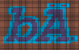
Fig. 17.4. ( Left ) The image R that is obtained by erosion between the image and the filter
shown in Fig. 17.3. The light red , representing 1, and the light blue representing 0, show
the changes introduced by the erosion. ( Right ) The image S that is obtained by a pointwise
multiplication between the left image and the right image of Fig. 17.2

17.2 Connected Component Labelling

For convenience, let 0 represent the color of the background. A connected compo-
nent is the collection (region) of all points having the color 1 such that they are
attached, i.e., if two points of the region are not already neighbors, there is a path
through neighboring points belonging to the region that can join any two points of
the region. We assume 8 -connected neighbors,

N 8 ( r k ) , for convenience but a 4-
connected 2 neighbors assumption is also possible. Evidently, in 3D binary images,
the neighborhood assumptions are more complex, because a point in a discrete 3D
image, called a voxel, can have face, edge, and vertex neighbors. We refer to [34, 35]
for a detailed discussion of binary image processing in higher dimensions. To fix
the ideas, a connected component is typically a region, also called an object, which
has one closed boundary with pixels having the same color. However, more than one
closed boundary is possible, e.g., the letter “e” in Fig. 17.5. Accordingly, it is pos-
sible to assign a unique label to each component. For simplicity one can use colors
to represent the labels e.g., as in Fig. 17.5. A method achieving this task is called
connected component labelling . This is not just an image-understanding problem but
also a computational physics problem, e.g., [7].
There are several techniques achieving connected component labelling [213] in
2D, differing in computational efficiency and computer architectures for which they
are intended. The differences are at the implementation level because there is, given
the neighborhood type, noroom for ambiguity on whether or not the labelling has
been achieved correctly. We outline the conventional method of doing such a la-
belling in 2D below because of its simplicity although there are other ways of achiev-
ing connected components labelling that may be more efficient [213].
The algorithm in [95] scans through a binary image f ( r i ) in the forward and the
backward raster directions alternately. Assume that f ( r i ) is a 2D (discrete) image
2 In 4 -connected neighbors, N 4 ( r k ), only points that share an edge with a pixel as neigh-
bors, i.e., top, down, left, and right pixels, are neighbors. An 8-connected neighborhood
assumption admits, additionally, the adjacent 4-diagonal pixels.