Image Processing Reference
In-Depth Information
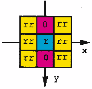
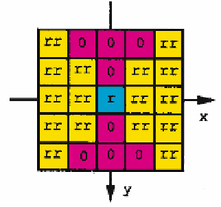
Fig. 16.6.
The coefficients of a butterfly filter with orientation
θ
=0for a 3
×
3 (
left
) and
5
×
5 (
right
) neighborhood
z
=
(
Γ
)
∗
g
(16.10)
where
Γ
is the image of labels,
(
Γ
) is the squared complex image (
D
x
Γ
+
iD
y
Γ
)
2
,
and
g
the convolution with an averaging filter. The argument of
z
obtained at every
pixel location represents
∗
arg(
z
)=
two
arg(
k
min
) (16.11)
where
k
min
is the complex number whose argument is the dominant boundary gra-
dient direction. In this case, the magnitude of the gradient of
Γ
is 1 at the transition
between two classes, and 0 within a class. The smoothing filter
g
is of size
s
s
and is
given by a Gaussian, which in this presentation is
s
=7induced by use of
σ
=1
.
8.
The direction is computed for the boundary pixels at the parent node level and is
propagated to the children level. For each dominant local direction, a butterfly-like
filter is defined. The butterflylike shape, Fig. 16.2, reduces the influence of vectors
along the boundaries that have high uncertainty. The shape and the weights of a 3
×
×
3
and 5
5 filter for the horizontal direction (
θ
=0) are given in Fig. 16.6, where
r
is a
function of the dissimilarity
d
, described below, between the two classes that define
the boundary and
rr
=(1
×
r
)
/N
ν
with
N
ν
being the number of weights different
from 0 or
r
. The dissimilarity
d
is given by
−
μ
m
−
μ
m
|
|
d
=
(
σ
m
)
2
+(
σ
m
)
2
(16.12)
where
μ
m
,μ
m
and (
σ
m
)
2
,
(
σ
m
)
2
are the means and the variances of the two classes
on both sides of the boundary in the
m
th component image of the feature vector
f
(
r
k
,l
). Note that the latter can be viewed as consisting of
M
layers of (scalar)
images. Then
r
=
r
(
d
) is defined empirically as an increasing function, here as in
Fig. 16.7 [229]. If the dissimilarity
d
is large then
r
=1and no smoothing is applied,
whereas a stronger smoothing is performed (
r
=
rr
) for low values of
d
.