Image Processing Reference
In-Depth Information
7
1
10
5
300
9
2
6
4
3
200
100
Left
Z
X
0
100
1000
Y
Z
Right
800
0
600
X
200
400
400
200
Y
600
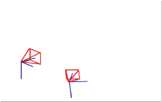
Fig. 13.8. This computed view of camera and checkerboard positions of Fig. 13.4 requires
knowledge of
M
E
,
M
I
,
M
I
, which are in turn computed by using known correspondence
points
to pull out
(
−−−→
O
W
P
)
W
=
R
L
T
(
−−−→
O
L
P
)
LC
−
R
L
T
t
L
(13.79)
and to obtain
p
by homogenization as
O
W
P
)
WH
=
(
−−−→
=
R
L
T
(
−−−→
(13.80)
p
=(
−−−→
R
L
T
t
L
O
W
P
)
W
1
O
L
P
)
LC
−
1
By substituting this in Eq. (13.71) and using the decomposition of
M
E
in analogy
with Eq. (13.77), we obtain:
T
R
M
R
p
=
T
R
M
I
M
E
p
=
T
R
M
I
[
R
R
,
t
R
]
R
L
T
(
−−−→
O
L
P
)
LC
−
R
L
T
t
L
1
=
T
R
M
I
(
R
R
(
R
L
T
(
−−−→
R
L
T
t
L
)+
t
R
)
O
L
P
)
LC
−
=
T
R
M
I
(
R
R
R
L
T
(
−−−→
R
R
R
L
T
t
L
+
t
R
)
O
L
P
)
LC
−
(13.81)
We now define,
R
=
R
R
R
L
T
,
t
=
t
R
Rt
L
,
−
and
M
E
=[
R
,
t
]
,
(13.82)
and call the matrix
M
E
the
stereo extrinsic matrix
because it represents the relative
rotation and displacement of the two cameras. Using Eq. (13.81) we then obtain the
equation of the right camera system as
T
R
M
R
p
=
T
R
M
I
(
R
(
−−−→
O
L
P
)
LC
+
t
)
=
T
R
M
I
[
R
,
t
]
p
=
T
R
M
I
M
E
p
(13.83)