Image Processing Reference
In-Depth Information
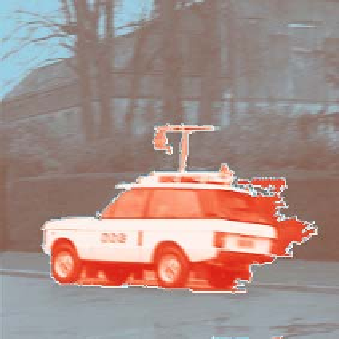
Fig. 12.5. Affine motion is estimated from 5 images (
right
) [61], using the eigenvectors of
(12.92). One of the original frames is shown on the
left
.Onthe
right
, the
red
car region, and
the
cyan-labeled
background region have different affine motion parameters which were found
automatically
freedom in the affine model. Naturally, more complex flow fields can be modeled by
the affine model than the translation model, which has only two degrees of freedom.
The affine matrix
A
0
can be decomposed into [58, 64, 132],
A
0
=
A
s
+
A
r
0
+
A
h
0
+
A
h
0
(12.83)
0
where the matrices on the right side control the amounts of rotation, scaling, shearing
of the first type, and shearing of the second type, respectively.
=
s
0
0
s
,
=
0
,
=
h
1
,
=
0
h
2
h
2
r
r
0
−
0
A
s
0
A
r
0
A
h
0
A
h
0
0
−
h
1
0
The CT in Eq. (12.81) is a differential equation modeling the speed or the optical
flow field, because
s
∗
−
s
δt
→
d
s
dt
=
v
(
x, y, t
)
(12.84)
when
δt
approaches to zero. Accordingly, the trajectory of a point in the image plane,
s
(
t
)=(
x
(
t
)
,y
(
t
))
T
, can be solved analytically. The six parameters represented by
v
0
and
A
0
steer the tangent curves of
s
. It can be shown that a small motion along
these curves can be achieved by an
affine infinitesimal operator
9
[58],
7
D
ζ
=
k
1
D
ξ
1
+
k
2
D
ξ
2
+
···
k
7
D
ξ
7
=
k
j
D
ξ
j
(12.85)
j
=1
9
The CT generated by the affine model is a Lie group of transformations of one parameter,
time.