Image Processing Reference
In-Depth Information
4
1
3
2
0.8
1
0.6
0
−1
0.4
−2
0.2
−3
−4
0
0.3
0.4
0.5
0.6
0.7
0.8
0.9
1
0.4
0.45
0.5
0.55
0.6
0.65
0.7
0.75
0.8
0.85
0.9
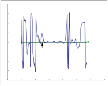
Fig. 10.27. The same as in Fig. 10.26 but the graphs on the
left
represent angle estimations
on the line joining point 5 to the center (
green
) and on the line joining point 6 to the center
(
blue
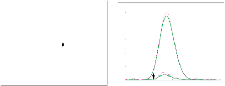
) marked in Fig. 10.15. In the
right
image, the two curves at the top, and the two curves at
the bottom represent
|I
20
|
(
solid curves
), and
I
11
(
dashed curves
) for two parts of the image.
The measurement pair on the top originates from the line joining point 5 to the center (clean),
whereas the pair at the bottom represents the measurements for the line between point 6 and
the center (noisy)
tions are evidently not Cartesian-separable, but the image can be rotated with fixed
increments, and the same horizontal set of filters can be applied. The result is rotated
back with the same amount. A disadvantage is that the filters, which are Gaussians,
give the same weight to low and high frequencies within the frequency cell they are
placed.
10.14 Relationship of the Two Discrete Structure Tensors
The structure tensor measures the second-order moment properties of the power
spectrum. It estimates the most prominent direction of the image in the TLS sense
and provides estimates on the quality of the fit. As we saw in Sect. 10.11, the tensor
can be directly discretized or, as in Sect. 10.13, first the spectrum can be discretized
via a Gabor filtering and then the structure tensor is computed for the discrete spec-
trum. Either case yields a discrete structure tensor that represents how well a TLS
fit of a line models the image spectrum. Below we discuss the relationship of both
techniques and the advantages of each.
The Gabor decomposition used in Sect. 10.13 to estimate the structure tensor
sampled the spectrum at just six points (only three filters were needed though!) along
a ring. According to the sampling theory discussed in Sect. 9.6, a sampled signal
must be lowpass filtered before sampling to deter sampling artifacts. This is, in fact,
done by the Gabor decomposition by a smoothing of the spectrum before sampling.
Suppose that we have a perfectly linear symmetric image, for the sake of discussion
a sinusoid in the spatial domain, with a crisp direction. This has a spectrum that has a
pair of Dirac pulses. As the direction of the image changes in the spatial domain, the