Image Processing Reference
In-Depth Information
0.4
0.4
0.5
0.5
0.6
0.7
0.8
0.9
0.8
0.7
0.6
0.6
0.7
0.8
0.9
0.8
0.7
0.6
1
1
5
2
4
6
5
2
4
6
3
3
0.5
0.5
0.4
0.4
0.5
0.7
0.9
0.7
0.5
0.5
0.7
0.9
0.7
0.5
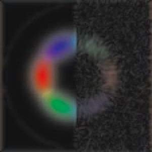
Fig. 10.25. The images illustrate the direction tensor, represented as
I
20
(
left
)and
I
11
(
right
),
for Fig. 10.15 and computed by using theorem 10.4 for Eqs. (10.87)-(10.89). The hue encodes
the direction, whereas the brightness represents the magnitudes of complex numbers. There
were three different tune-on directions in a set of three Gabor filters
(radians). The arrows show the limits of the frequency annulus to which the Gabor
filters are most sensitive, as confirmed by the graphs of
and
I
11
in the right. The
main disadvantage of this direction estimation compared to the one presented in Sect.
10.11 is due to the poor quality estimations, caused by the very coarse discretization
of the spectrum in three directions. The accuracy of the direction estimation itself
is, however, fully sufficient for many applications. Both direction accuracy and error
estimation accuracy can be improved significantly by a nonminimalist set-up of the
Gabor decomposition. This will be elaborated in the next section further. Here, we
wanted to show that even with three Gabor filters it is possible to obtain reasonably
accurate estimates of the direction, albeit the error estimates of the directions are not
nearly as good.
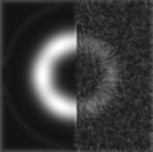
|
I
20
|
Structure Tensor by Cartesian Gabor Decomposition
It is worth noting that the local spectrum must not be sampled via a separable tessel-
lation in the orientation and the absolute frequency, although such a decomposition
has advantages for pattern recognition purposes. The algorithm represented by Eqs.
(10.84)-(10.85) will still hold for reasonably densely discretized power spectra, in-
cluding a Gabor filter bank that covers the frequency plane in a Cartesian-separable
fashion, as shown in Fig. 10.28. In this graph the tuning frequencies of the filters
(marked with
) along with the iso-amplitude curves of the filters are shown (the red
and the cyan curves). For real images, half of the filters are not used, those drawn
with cyan in the graph, as before because they are deducible from the other half. The
dashed and solid axes show two example frequency responses at which the spectral
energy will ideally be concentrated if the image is linearly symmetric having a gra-
×