Image Processing Reference
In-Depth Information
0.4
0.5
0.6
0.7
0.8
0.9
0.8
0.7
0.6
1
5
2
4
6
3
0.5
0.4
0.5
0.7
0.9
0.7
0.5
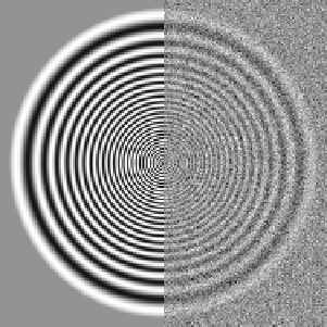
Fig. 10.15. On the
left
, the test image, the axes of which are marked with fractions of
π
representing the spatial frequency. On the
right
is the color code representing the directions.
The marks on the axes are separated by 5 degrees when joined to the center. The
colored dots
in both images define the curves from which 1D direction measurements will be sampled
The integral represents a continuous convolution, and Eq. (10.73) is obtained by
noting that both
μ
and
w
are Gaussians and that a convolution of them yields another
Gaussian, with a variance that is the sum of the variances of
μ
and
w
. An easy way
of seeing this is by applying the Fourier transform to
μ
w
. Eq. (10.72), which
computes the local tensor around the origin, is therefore a discrete convolution by
a Gaussian if
S
(
i, j
) needs to be computed for local patches around
all
points of
the original im
age grid
. Since the values of
μ
l
s decrease rapidly outside of a circle
∗
with radius
σ
p
+
σ
w
, we can truncate the infinite filter when its coefficients are
sufficiently small, typically when the coefficients have decreased to about 1% of
the filter maximum. Thus, Eq. (10.72) implies that the local tensor (of the origin) is
obtained as a window-weighted average of the gradient outer products:
1
4
π
2
f
l
)
T
μ
l
S
=
(
∇
f
l
)(
∇
(10.74)
l
where
f
l
is the gradient of
f
(
r
) at the discrete image position
r
l
, and
μ
l
is a discrete
Gaussian. Defining
D
x
f
l
and
D
y
f
l
, for convenience, as the components of
∇
∇
f
l
,at
the mesh point
r
l
:
=(
∂f
(
r
l
)
∂x
,
∂f
(
r
l
)
∂y
f
l
=(
D
x
f
l
,D
y
f
l
)
T
)
T
,
∇
(10.75)
We summarize our finding on tensor discretization as a theorem:
Theorem 10.3 (Discrete structure tensor I).
Assuming a Gaussian interpolator
with
σ
p
and a Gaussian window with
σ
w
, the optimal
discrete structure tensor
ap-
proximation is given by