Image Processing Reference
In-Depth Information
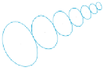
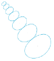
Fig. 9.15. The isocurves of Gabor filters at cell boundaries. The orientation and frequency
resolution of the decomposition are explicitly controllable because the frequency cells are
designed in the log(
z
) coordinates
ξ
n
)=exp
ξ
n
2
2
σ
ξ
−
ξ
−
G
n
(
ξ
)=
W
(
ξ
−
(9.49)
where
ξ
n
and
σ
ξ
are tune-on and bandwidth parameters as before, but in the mapped
frequency, i.e., the
ξ
-domain. These filters can be remapped to the
ω
-domain via
ξ
n
]=exp
−
ξ
(
ω
)
−
ξ
n
2
2
σ
ξ
G
n
[
ξ
(
ω
)] =
W
[
ξ
(
ω
)
−
(9.50)
where
ξ
(
ω
) is the log function given by Eq. (9.48). As illustrated by Fig. 9.14, the
only difference in this approach is the transformation Eq. (9.48) applied to the
ω
-
coordinate, which enables the filters to be designed in the
ξ
-domain such that they
all become identical and ordinary Gaussians translated to the centers of equally sized
cells. The function
G
n
(
ξ
(
ω
)) vanishes at
ω
=0, which guarantees that these fil-
ters have no DC bias, as opposed to
G
n
(
ω
)
>
0 at
ω
=0, discussed in the pre-
vious section. The filter bank uses the same parameters as the one illustrated by
Fig. 9.13. Note that there are more resources (filters) devoted to the low-frequency
range where humans are most sensitive. More precisely, the tune-on frequencies, the
cell-boundaries, as well as the bandwidths, defined as the size of cells in
ω
-domain,
progress geometrically with the factor (
ω
max
/ω
min
)
Ω
ξ
, with
Ω
ξ
being the cell size.