Image Processing Reference
In-Depth Information
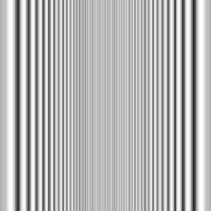
Fig. 8.8. A 1D function (a line) containing slow and rapid gray changes is translated with
zero shifts (
left
) and 0.67 points (noninterpolated) shifts (
right
) between successive lines. Each
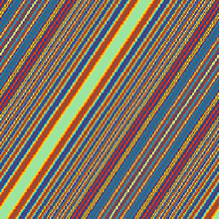
color represents a unique gray level of the original, which is given in color in Fig. 12.4 along
with the interpolated shifts. The
vertical axis
is time
The result is a scalar product between the shifted, sampled interpolation function,
which easily lends itself to be implemented as a convolution.
If this scalar product is not implemented, translation will result in aliasing effects.
This is illustrated for 1D functions by Fig. 8.8, where we show 1D functions as lines
of an image. The image on the left is obtained by repeating the same line (the 1D
function), i.e., the translation is zero between the successive lines. We applied 0.67
pixels (cyclical) translation to the same 1D function to obtain the successive lines,
by rounding off 0
.
67
j
where
j
is the horizontal index, of the image on the right.
Apart from the jaggedness of the lines, we also see erroneous gray levels in the
high-frequency parts, where both aliasing problems are due to the straightforward
implementation of the translation. This should be compared to Fig. 12.4 (top and
middle), where we show the translation performed according to Eq. (8.20), which
contains interpolation.
Note, however, when one produces a (higher dimensional)
motion image
by suc-
cessive application of a translation to a static image
f
, such as the one in the example,
the resulting image will potentially have a large
temporal
frequency extent as well.
This extent depends on the size of the shift as well as on the frequency content of
the static pattern
f
. Because the temporal frequencies must obey the law of sampling
to avoid the errors of discretization, for every temporal sampling frequency there is
a maximum speed/shift that should not be exceeded. The implications of motion on
the spectrum are discussed in further detail in Sect. 12.7.
In conclusion, a linear band-preserving continuous operator can be discretized by
discretizing the result of the operator applied to the interpolation function in analogy
with the partial derivative operator.