Image Processing Reference
In-Depth Information
1.8
1
1.6
1.4
0.8
1.2
1
0.6
0.8
0.4
0.6
0.4
0.2
0.2
0
0
−4
−3
−2
−1
0
1
2
3
4
−4
−3
−2
−1
0
1
2
3
4
1.6
1.6
1.4
1.4
1.2
1.2
1
1
0.8
0.8
0.6
0.6
0.4
0.4
0.2
0.2
0
0
−4
−3
−2
−1
0
1
2
3
4
−3
−2
−1
0
1
2
3
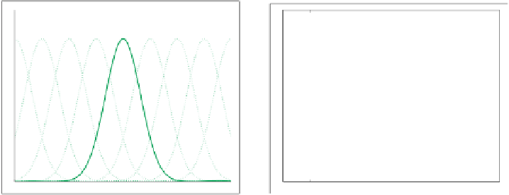
Fig. 8.7. (
Top, left
) The graph illustrates a set of Gaussians, with
σ
=0
.
65, that are used as
differentiable interpolators. (
Top, right
) Summing up the interpolators approximates a constant
function. (
Bottom, left
) A function to be approximated (the same as in Fig. 8.6) along with an
interpolator amplified by its function sample. (
Bottom, right
) The
green curve
is the result of
the approximation, the normalized sum of the amplified interpolators
Partial Derivatives
In image analysis, the partial derivative of a function, which is only discretely avail-
able, is a frequently demanded operation that ideally should also result in a discrete
image. Ideally, the computations performed on the discrete samples of the image
should result in a discrete version of the result delivered by the continuous opera-
tor applied to the continuous image. To take the partial derivative of a function is
evidently linear because
∂
∂x
(
f
+
g
)=
∂
∂x
(
f
)+
∂
∂x
(
g
)
,
∂
∂x
(
λf
)=
λ
∂
∂x
(
f
)
.
and
(8.16)
The partial derivative is one of the most frequently used operators in image pro-
cessing, e.g., to extract edges, lines, direction, curvature, and texture properties. In
particular, arbitrary
partial derivatives
of a differentiable scalar function
f
(
r
), where
r
=(
x
1
,x
2
,
∂f
(
r
)
∂x
j
x
N
)
T
, are represented by
···
with
j
=1
,
2
,
···
N
. The function