Image Processing Reference
In-Depth Information
1
1
0.8
0.8
0.6
0.6
0.4
0.4
0.2
0.2
0
0
−4
−3
−2
−1
0
1
2
3
4
−4
−3
−2
−1
0
1
2
3
4
1.6
1.6
1.4
1.4
1.2
1.2
1
1
0.8
0.8
0.6
0.6
0.4
0.4
0.2
0.2
0
0
−4
−3
−2
−1
0
1
2
3
4
−3
−2
−1
0
1
2
3
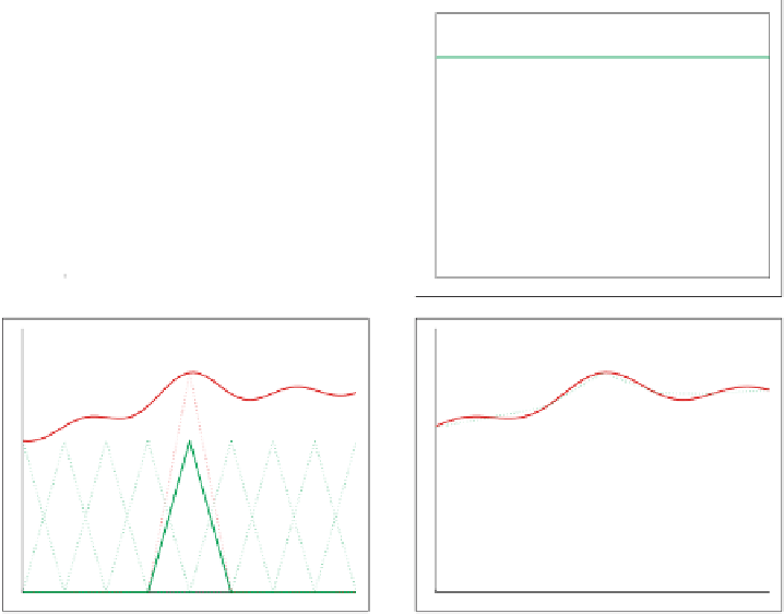
Fig. 8.6. (
Top, left
) The graph illustrates the set of linear interpolators on a discrete set of
points. (
Top, right
) Summing up the interpolators, approximates the constant function 1. (
Bot-
tom, left
) A function to be approximated along with an interpolator amplified by its function
sample. (
Bottom, right
) The green curve is the result of the approximation, the sum of the
amplified interpolators
Assume that we are given a set of function values
f
(
r
l
), where
r
l
is a discrete set
of points that we will call
grid
. From this, the continuous
f
(
r
) can be synthesized by
using Eq. (8.6)
f
(
r
)=
l
f
(
r
l
)
μ
(
r
−
r
l
)
(8.15)
with
μ
being an interpolation function. This continuous
reconstruction
is merely
a mental process that is done to implement continuous linear operators discretely.
Ultimately, we wish to be able to implement every continuous operator discretely.
However, there is no effective formula that will fit all types of operators. Instead, we
aim here to illustrate how to implement some frequently occurring linear continuous
operators, in particular, those that do not change the bandwidth of the functions. The
latter is an important restriction that raises the hope of success because we can always
represent every function with finite frequencies well enough by its samples. We illus-
trate the technique by showing how to implement partial derivation and noninteger
shifts on a discrete grid.