Biomedical Engineering Reference
In-Depth Information
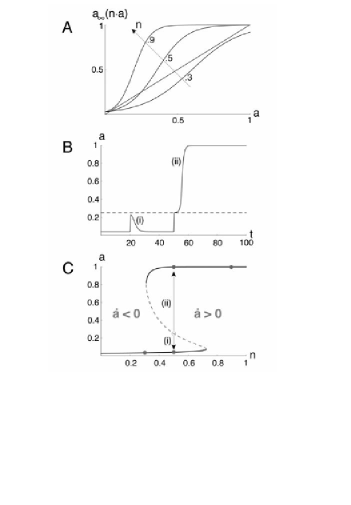
Figure 3
. (
A
) Graphical solutions of the equation
a
=
a
(
n
#
a
). Depending on the value of
n
,
there can be 1 or 3 solutions. (
B
) Time course of network activity for
n
= 0.5. The network
receives external inputs at
t
= 20 and
t
= 50 (arbitrary unit normalized to U
a
). The first input (i)
brings the activity just below the middle state (network threshold, dashed line) so activity
decreases back to the low state. The second input brings activity just above the network thresh-
old, and then jumps up to the high steady state. (
C
) Diagram showing the possible steady state
values of activity for all values of
n
between 0 and 1. The dashed curve (middle branch) indi-
cates unstable states. The steady states determined in A are represented on the curve by filled
(stable) or open (unstable) circles. Modified from Tabak et al. (36).
intersection for a low value of
a
. Thus, the connectivity is too small to sustain a
high level of activity. Even if the network is transiently stimulated, activity will
quickly go back to its low level state. On the other hand, for large values of
n
(
n