Geology Reference
In-Depth Information
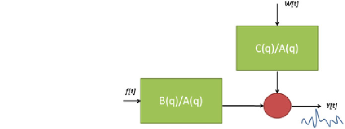
Fig. 4.2 Block diagram of
the ARMAX model
model contains p autoregressive terms, q moving average terms, and r exogenous
inputs terms as follows in the equation
X
p
X
q
X
r
l¼o
g
l
w
y
i
ð
Þ
¼
a
j
y
i
ð
Þþ
ð
Þþ
ð
Þþ
e
i
ð
Þ
ð
4
:
13
Þ
t
t
j
b
k
f
t
k
t
l
t
j¼1
k¼o
where w(t) is the known external time series (inputs),
g
l
is parameters of the
exogenous input d, and f(t) is a reference signal. Other notations are as described in
the previous section.
4.2 Local Linear Regression Model
The LLR technique is a widely studied nonparametric regression method which
provided very good performances in many low dimensional forecasting and
smoothing problems. The advantage of LLR technique is that it does not require a
long time series for the development of a predictive model. A reasonably reliable
statistical modeling can be performed locally with a small amount of sample data. At
the same time, LLR can produce very accurate predictions in regions of high data
density in input space. These are the major attractions of LLR and have gained
considerable attention among researchers, who acknowledge LLR as a very effective
interpolative tool. The LLR procedure requires only three data points to obtain an
initial prediction and then uses all newly predicted data as it becomes available to
make future predictions. The only problem with LLR is to decide the size of p
max
, the
number of near neighbors to be included for the local linear modeling. The method of
choosing p
max
for linear regression is called in
uence statistics. A trial and error
process to determine the value of in
uence statistics was carried out.
Given a neighborhood of p
max
points, the linear matrix equation must be solved:
Xm
¼
y
ð
4
:
14
Þ
where X is a p
max
d matrix of
the p
max
input points in d-dimensions,
x
i
ð
1
i
p
max
Þ
are the nearest neighbor points, y is a column vector of length p
max