Geology Reference
In-Depth Information
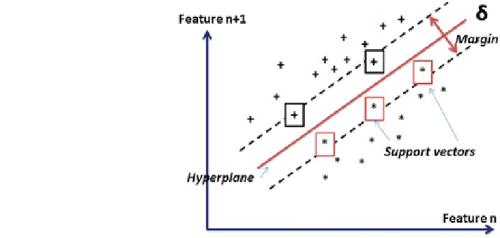
Fig. 4.15 Separation of
hyperplane in SVM modeling
As we are interested only in support vector regression (SVR), we can look into
its mathematical details.
Let data examples [(x
1
, y
1
), (x
2
, y
2
),
,(xi, yi)] be a given training set, where
xi denotes an input vector, and yi is its corresponding output data set. SVR maps
x into a feature space via a nonlinear function
…
Φ
(x), and then
finds a regression
function f(x)=w
·
Φ
(x)+b which can best approximate the actual output y with an
error tolerance
, where w and b are the regression function parameters known as
weight vector and bias value, respectively.
ε
is known as a nonlinear mapping
function [
17
]. Based on the SVM theorem, f(x) can solve problems as shown below:
Φ
1
2
j
C
X
N
minimize
w
2
1
ðn
k
þ n
k
Þ
j j
w
þ
ð
4
:
55
Þ
; n; n;
;
b
k
¼
subject to
8
<
:
9
=
;
y
k
w
T
/
X
ðÞ
b
eþn
k
e þ n
k
w
T
/
X
ðÞþ
b
y
k
k
¼
1
;
2
;
3
...
N
ð
4
:
56
Þ
n
k
n
k
0
In the above equation, C is a positive trade-off parameter which determines the
degree of error in the training stage and
ξ
and
ξ
* are slack variables which penalize
training errors by Vapnik
'
s
ξ—
insensitivity loss function. In the optimization
2
improves the generalization of the SVM by regulating the
degree of model complexity. The C
P
k¼1
n
k
þ n
k
equation, the term
2
j
j j
w
controls the degree of
empirical risk. Figure
4.16
illustrates the concept of SVR. The above equation can
be reformulated to dual form using Lagrangian multipliers (
ʱ
,
ʱ
*):