Model Urbanization Strategy: Summaries, Recommendations and Requirements - Meteorological and Air Quality Models for Urban Areas - page 139

The simplest approaches, which include the traditional Reynold's averaging
scheme (using roughness and displacement length), are single-layer schemes that
link the UC effects to the atmospheric boundary layer through the model's lowest
layer. In these methods, the urban scheme is implemented through parameterization
of each grid's radiative and turbulent flux values. Moreover, details regarding drag
aspects typically are addressed through various ad hoc approaches. For example,
simple analytical wind profile formulations for applications inside the canopy typ-
ically are introduced. Removing this limitation requires implementation of urban
schemes with multi-layers in which the flux quantities interact with the atmospheric
variable (Martilli et al., 2002; Dupont et al., 2004). This approach requires addi-
tional terms in the prognostic equations of the atmospheric models (e.g., drag term
in momentum equations, heating term in temperature equations, production term in
turbulent kinetic energy equations). Such models require the addition of layers from
the surface to the top of the highest urban feature, thus representing the morpholog-
ical features as functions of height for each grid. This allows the schemes to model
the interactions between air and the urban environment at several heights. Thus, it
is possible to simulate the in-canopy flows with greater precision than in single-
layer models. However, additional prognostic equations and vertical model levels
are required for this type of implementation. Consequently, whereas the effects of
surface features are better represented, the computation burden is increased because
of the increased integration time step and treatment of additional modeling details.
This additional burden presents a limit in the use of multilayer canopy models in
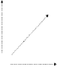
NWP forecasting. Clearly, as seen in Fig. 15.1, care must be taken at the outset to
understand and balance the need for greater precision obtainable with full canopy
details and model turnaround time.
Too expensive to run?
Globally more
applicable?
Parameters difficult
to get?
Number of Parameters
Fig. 15.1 Schematic diagramme depicting computational requirement increases with the inclu-
sion of increased levels of UCP sophistication in UC models (from workshop presentation by
Grimmond et al. (Chapter 11) of this volume)