Environmental Engineering Reference
In-Depth Information
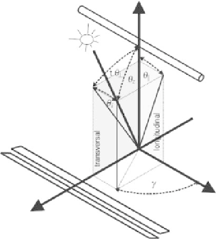
Figure 14.3.13
Angles definition of a linear Fresnel reflector with horizontal N-S orientation tracking
axis (Mertins, 2009).
For simplicity, the overall IAM of the collector is calculated as the product of two
different IAMs related to
θ
||
and
θ
⊥
characteristic incidence angles, as follows:
IAM
(
θ
z
;
γ
)
=
IAM
(
θ
⊥
)
·
IAM
(
θ
i
)
(14.3.13)
This methodology was introduced by McIntire (1982) and Ronnelid et al. (1997) and
recently confirmed by Mertins (2009). As an example, the IAM (
θ
i
) and IAM (
θ
⊥
)
of a commercial collector are shown in Figure 14.3.14. These data are taken from a
commercial simulation tool (Thermoflex® database). From the result, it can be noted
that IAM (
θ
i
), which is not the tracking axis, gives the larger contribution to the IAM,
while IAM (
θ
⊥
) exhibits an irregular trend for incidence angles between 0
◦
and 45
◦
because of the secondary reflector shading over primary mirrors, reducing effective
mirror aperture area.
To summarize, the optical efficiencies of LFR are defined as:
η
optical
_
LFR
=
η
optical
_
LFR
|
0
◦
IAM
(
θ
⊥
)
IAM
(
θ
i
)
θ
end
_
loss
(14.3.14)
The LFR optical efficiency ratio shown in Figure 14.3.15 summarizes the optical effi-
ciency of the collector for every month of the year. IAM (
θ
i
) presents a maximum
during the day at 10 h and 16 h, while the presence of IAM (
θ
⊥
) in LFR leads to a
smoother shape, with lower efficiency, in particular for high incidence angles. Com-
pared to a parabolic trough collector (see Figure 14.3.8), which is affected only by
θ
i
,
linear Fresnel has a lower optical efficiency.
Search WWH ::

Custom Search