Applications of Chemical Kinetics in Environmental Systems - Elements of Environmental Engineering: Thermodynamics and Kinetics - page 353

in ppmv or ppbv) by multiplying with 0.0224 m 3 CFC/mol, which is the molar volume
of CFC.
Letusfirstcalculatethevaluesof[CFC],[CFC] 0 ,and[CFC] ss fortheyear1987when
the Montreal Protocol took effect. In 1987, [CFC] ∼ 450 pptv for CFC-12. If we choose
k − 0.0065 y − 1 , a production rate for CFC-12 of Q s ∼ 3 × 10 9 mol/y, and V atm =
3.97 × 10 18 m 3 , we obtain [CFC] ss = 2.8 ppbv. If, further, we assume a constant Q s ,
then

[CFC]
[CFC] 0 = 6.2 − 5.2e − 0.0065 t .
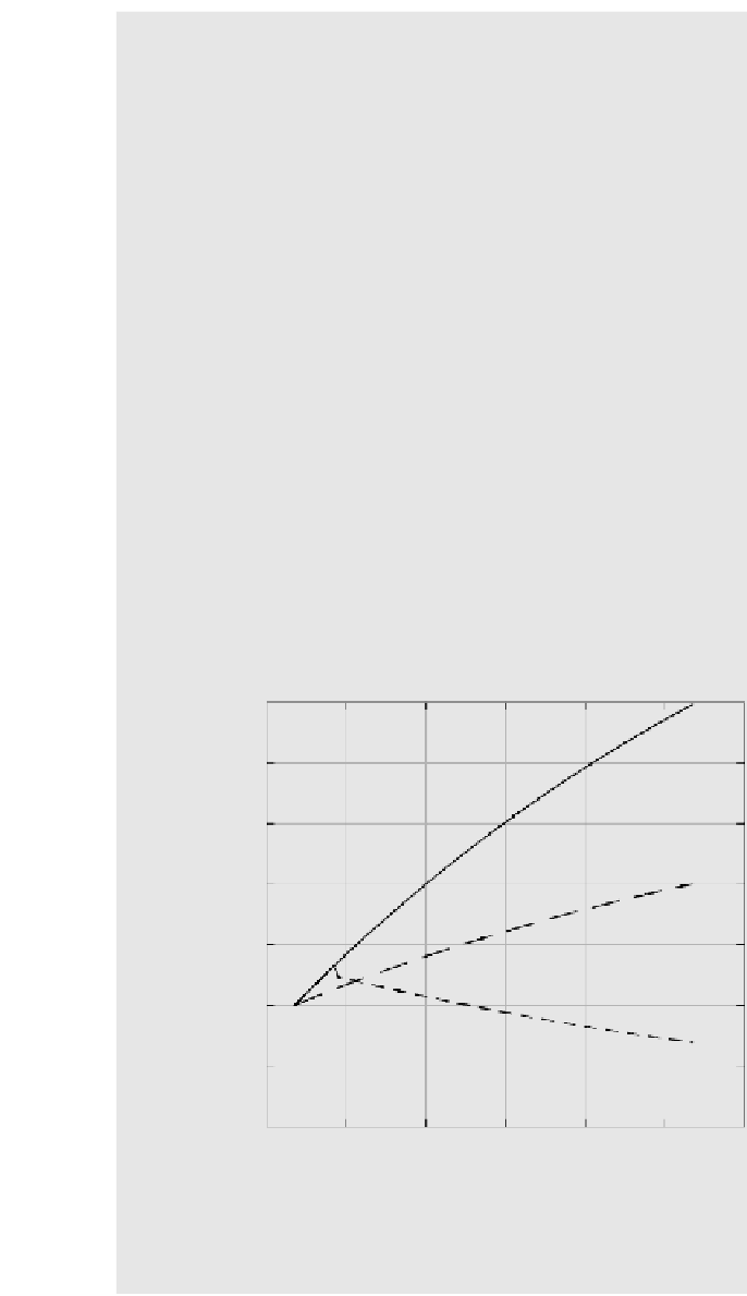
Curve 1 of Figure 6.48 shows the resulting profile. This can be considered to be the
base case , that is, a consequence of nonimplementation of the Montreal Protocol. If the
Montreal Protocol is to reach a goal of 50% reduction in net CFC emissions, then Q s
has to be replaced by 0.5 Q s and [CFC] ss = 1.4 ppbv. Hence,

[CFC]

[CFC] 0 = 3.1 − 2.1e − 0.0065 t .
Curve 2 of Figure 6.48 shows the expected CFC concentration in air in this case. Note
that even under this scenario, the CFC concentration continues to rise in the atmosphere,
albeit at a slower rate. As a consequence, chemical reactions causing the destruction
of stratospheric ozone will continue into the next century. Figure 6.48 also considers
the following scenario: What if the Montreal Protocol had attempted the complete
cessation of CFC production by 1997? The decay of CFC concentration will then be
given by

3.5

3

G 0

2.5

0.5 G 0

2

1.5

G = 0 in 1997

1

0.5

0

1980 2000 2020 2040 2060 2080 2100

Ye a r

FIGURE 6.48 Atmospheric concentration of CFCs for various scenarios of the
Montreal Protocol.

continued