Concepts from Chemical Reaction Kinetics - Elements of Environmental Engineering: Thermodynamics and Kinetics - page 251

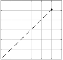
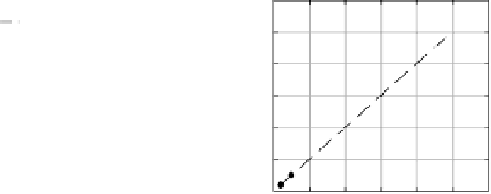
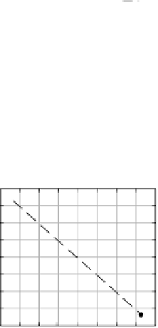
The three plots for the above data are shown in Figure 5.20. The values of K m
and V max obtained are given below:

r 2

Method K m /mM V max /mM/min

Lineweaver-Burke 0.9999 10.1 20.0

Langmuir 0.9998 10.0 19.9

Eadie-Hofstee 0.9986 10.0 19.9

Often the Lineweaver-Burke plot is preferred since it gives a direct relationship
between the independent variable [S] and the dependent variable r . There is one short-
coming, that is, as

, and hence is inappropriate at low [S]. The value
of the Eadie-Hofstee plot lies in the fact that it gives equal weight to all points unlike
the Lineweaver-Burke plot. In the present case, the Lineweaver-Burke plot appears to
be the best.

[ S ]→ 0, 1 /r →∞

Langmir Plot

Lineweaver-Burke Plot

0.0035

(a) (b) 0.35

y = 0.00050409 + 0.050194 x R 2
= 0.99988

y = 0.049933 + 0.00050611 x R 2
= 0.99991

0.003

0.3

0.0025

0.25

0.002

0.2

0.15 0.0015

0.1 0.001

0.05 0.0005

0 100 200 300 400 500 600 0 0.01 0.02 0.03 0.04 0.05 0.06

1/[S]/M -1 [S]/M

Eadie-Hofstee plot
y = 19.932 - 0.010049 x R 2
= 0.99859

(c)

18

16

14

12

10

8

6

4

2

200 400 600 800 1000 1200 1400 1600 1800

r /[S]/mM/M.min -1

FIGURE 5.20 Estimation of Michaelis-Menten parameters using different methods.
(a) Lineweaver-Burke plot, (b) Langmuir plot, and (c) Eadie-Hofstee plot.

Michaelis-Menten kinetics considers the case where the number of living cells
producing the enzymes is so large that little or no increase in cell number occurs. In
other words, the Michaelis-Menten law is applicable for a no-growth situation with