Image Processing - Practical Rendering and Computation with Direct3D 11 - page 466

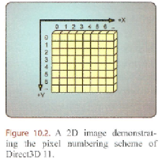
of a signal, which is sampled at uniformly spaced
sample locations. Each sample in the image is re-
ferred to as a pixel, and can contain up to four com-
ponents to represent the sampled signal value at the
location of a given pixel. All pixels within an image
share the same value format. This description goes
along with the familiar 2D grid that is commonly
used to show an image, as seen in Figure 10.2,
which shows the pixel addressing scheme used by
Direct3D 11.
It is also noteworthy that there is no restric-
tion to an image being two dimensional. There are
many image processing algorithms that can be per-
formed on ID, 2D, 3D, or even higher dimensional signals. However, since the focus of
this topic is on real-time rendering, we will restrict the discussion to 2D image processing
algorithms.

10.1.2 Image Convolution

With this basic definition of an image, we can look a little deeper into the nature of how
image processing algorithms function. Many filtering algorithms are implemented as a
convolution between the input image itself and another function, referred to as a filtering
kernel. For discrete domains like our images, the convolution operation is defined as shown
in Equation (10.1):

(10.1)

This mathematical definition may seem some-
what complex at first, but if we take a simplified
view of it, we can more clearly see how this op-
eration is applied to images. The convolution is an
operation which takes two functions as input and
produces an output function. In our image-process-
ing domain, this means that each pixel in the output
image is calculated as the summation of the product
of the two input images' pixels at various shifted
locations. The shifted locations make the two im-
ages conceptually move with respect to one another
as each pixel is being processed. To visualize this

Figure 10.3. The conceptual view of an
input image and the filter kernel during
processing of a single pixel.