Dynamic Tessellation - Practical Rendering and Computation with Direct3D 11 - page 442

Results
Figure 9.22 and Figure 9.23 demonstrate the difference made by the new algorithm.
Although Figure 9.22 may appear more aesthetically pleasing due to the smooth gra-
dients, the more chaotically shaded Figure 9.23 is by far the better image, from a geometric
perspective. In both images, the patch detail is translated into a color—red for high detail,
green for mid detail, and blue for low detail. Black is the lowest detail.
The lower half of each image is the corresponding wireframe representation, which
clearly and obviously shows the approximately 40% reduction in triangle count.
Consider the bottom center area of both image. In Figure 9.22 it is mostly shaded in
orange, whereas in Figure 9.22, it is predominantly black. It is also important to notice that
the surface being represented is flat for this section of terrain. The naive distance-based
calculation assigns this geometrically simple piece of terrain a high number of triangles,
although it simply doesn't need it. Why waste processing power and memory bandwidth
generating and rasterizing extra triangles that add nothing to the final image?
Examining Figures 9.22 and 9.23 initially suggests that the computer shader ap-
proach has greatly reduced the LOD across the whole image. This is based on the ob-
servation that most of the terrain tiles are shades of blue, while the majority are green
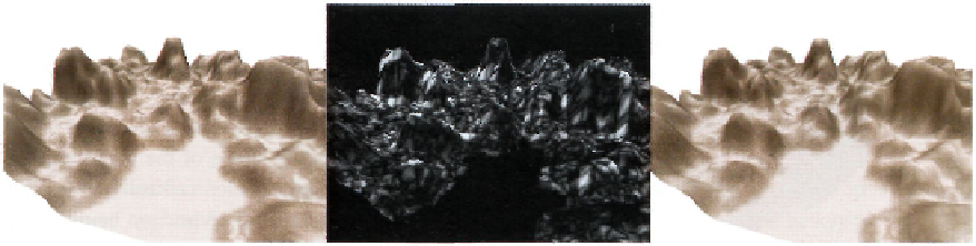
and yellow in the na'ive implementation. Figure 9.24 makes it easy to compare the naive
approach (on the left) and the computer shader approach (on the right).
When rendering is performed using a simple N*L directional lighting shader with
solid shading, we get an image much closer to what would be rendered in a real applica-
tion. The only major omission is the lack of textures (such as grass and rock). In addi-
tion to naive and computer shader approaches shown, the middle of Figure 9.24 shows
a simple image-based difference of the two results on either side. Here, black means no
difference, and white means that they are completely different. Comparing the rasterized
image is preferable to comparing the underlying geometry because ultimately, it is the
Figure 9.24. Comparison of naive and compute shader approaches.