Efficient LPC Quantization Methods - Digital Speech: Coding for Low Bit Rate Communication Systems - page 134

3850

f 10
g 10

3750

3650

3550

3450

3350

3250

0 500 1000 1500 2000

Time (samples)

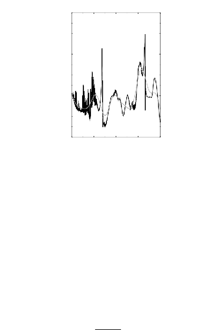
Figure 5.23 LSF tracks f 10 and g 10 variations over time

This advantage is shown in the following test. First, the classical method of
LSF extraction is applied at various update rates. Next, the low-pass filtered
method is used where LSFs are calculated at every sample. Each LSF track
is then filtered with a low-pass filter which had its cut off frequency suitably
selected to be half of the LSF transmission frequency. A subsampling is then
applied to get the required number of LSF vectors. Finally, the variance
for each set of LSF vectors is computed after a single-order MA prediction.
According to the earlier observations, the new method is expected to pro-
duce smaller prediction residual with a greater prediction coefficient owing
to its smoother evolution and hence higher correlation between successive
sets. Figure 5.26 shows that for a 20ms update rate, the variance of the LSF
prediction residual is lower for the new method and the minimum variance
(best prediction) occurs at a higher value of prediction coefficient which
indicates that the newmethod produces LSF vectors that are more correlated.
Figures 5.24-5.28 show similar results for various other LSF vector transmis-
sion rates. It can be seen that the variance of the LSF prediction residual is
always less in the new method, regardless of the LSF vector rate. In order to
quantify the amount of prediction achieved, prediction gain, P g ,iscomputed
using,

x 0 − x min

x 0

P g = × 100 (5.79)