Geology Reference
In-Depth Information
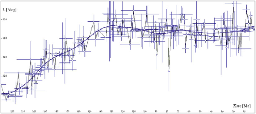
Fig. 6.12
Predicted paleolatitudes for a reference point
in N. America at (55
ı
N, 90
ı
W) since the late Triassic,
based on the global compilation of Schettino and Scotese
(
2005
). The regression curve is a natural cubic spline, built
using a smoothing parameter “
D
5
Jupp and Kent (
1987
) can be found in Torsvik
et al. (
1996
,
2012
). An alternative technique of
construction of smoothed APW paths has been
proposed more recently by Schettino and Scotese
(
2005
). This approach tries to overcome the limits
of the spherical splines smoothing algorithms,
in which the amount of smoothing is chosen
arbitrarily by the researcher, and the regression
may determine a best fitting curve that is not so
best with regard to the local geology at individual
sites. To understand the problem, let us consider
the plot of Fig.
6.12
, which shows the predicted
paleolatitudes of a point on the North American
craton since the late Triassic.
The plot in Fig.
6.12
has been built using
(
6.54
) and combining paleopoles from N. Amer-
ica with paleopoles from other continents, which
were rotated into N. American coordinates us-
ing the rotation model of Schettino and Scotese
(
2005
). We note that the overall trend of paleo-
latitude for the selected reference point is an ap-
proximately linear increase by
36
ı
from the late
Ladinian (230 Ma) to the Barremian (130 Ma),
then a more or less constant paleolatitude un-
til recent times. However, the smoothing spline
curve of regression, which has 4.8
ı
rms error of
residuals, shows a sequence of second-order low-
amplitude oscillations about the general trend.
These oscillations could be interpreted as real
cycles having geological significance. However,
if we used a greater smoothing parameter, say “
D
300, in order to generate a regression curve
that is more representative of the general trend,
the maximum displacement of the spline curve in
Fig.
6.12
from the new representative trend would
be only œ
D
3.3
ı
(Fig.
6.13
). Therefore, the
predicted paleolatitude oscillations would have
amplitude that is less than the standard deviation
of the residuals about the regression line!
This example can be extended to the spherical
regression curves that are used in the modelling
of APW paths. It shows that the smoothing
parameter of a spline regression curve cannot be
chosen arbitrarily, but it should be compatible
with the dispersion of the data about the
regression curve. Another more critical problem
of the “crude” statistical approach will be
discussed now. To this end, it will be useful
to examine in detail some key features of the
approach of Schettino and Scotese (
2005
).
These authors compiled a list of paleopoles for
each continent by filtering data in the GPMDB
according to some minimum-reliability criteria
(
B
4,
N
/
B
4,
A
95
15
ı
, cleaning procedure
code
2, and half-interval of age uncertainty
20 Myrs). In the analysis of a continent, the
paleopoles belonging to other plates were rotated
into the local coordinate system of the continent