Geology Reference
In-Depth Information
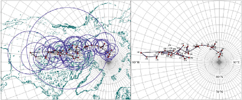
Fig. 6.10
A sliding-window APW path for the African
craton since 200 Ma (Besse and Courtillot
2002
), obtained
using a 10 Myrs window and 5 Myrs steps.
Blue circles
are
A
95
confidence cones (
left
).
Red dots
are mean paleopole
locations. The
right
pane shows more clearly the complex-
ity of this path, which includes several loops and hairpins
an APW path is a time series of
mean
paleopoles
p
(
t
1
),
p
(
t
2
), :::,
p
(
t
N
), where
t
1
<
t
2
<:::<
t
N
.
Therefore, a versor
p
(
t
i
) is always calculated
by a weighted averaging formula like (
6.55
).
Geometrically, the time series is represented by a
curve on the unit sphere, formed by a sequence
of great circle arcs linking the paleopoles. A
potential source of ambiguity in the construction
of these curves arises from the geomagnetic field
reversals. However, in paleomagnetic databases
like the GPMDB such ambiguity is overcome
by assigning to each listed paleopole a normal
polarity. Eventually, in the case of southern
hemisphere continents, it is possible to reverse all
the paleomagnetic poles and visualize the APW
paths as inverted polarity curves. The first APW
paths were built selecting groups of paleopoles
according to their
geologic
age. For example,
one could start determining the average of all
paleopoles having a stratigraphic or radiometric
age in the lower Cretaceous time interval,
obtaining the representative mean paleopole for
the lower Cretaceous. Then, the procedure was
repeated for the upper Cretaceous paleopoles,
and so on. This simple method was the only
possible approach when the number of available
paleopoles satisfying minimum reliability
criteria was small. Starting from the 1990s, the
publication of many new results allowed more
refined
Today, there are three general approaches to
the construction of APW paths. In the
sliding
window
method (e.g., Harrison and Lindh
1982
),
the paleomagnetic poles with ages falling within
a time window of fixed width (for example,
30 Myrs) are averaged to determine a mean
paleopole, which it is attributed an age equal
to the central age of the interval, or equal to
the mean age of the averaged paleopoles. Then,
the window is moved by an assigned step (for
example, 10 Myrs) and the procedure is repeated.
An example of sliding-window APW path is
shown in Fig.
6.10
.
A major problem with APW paths like that
illustrated in Fig.
6.10
is that they show a level of
detail higher than what is statistically justifiable.
This is quite evident by comparing the confidence
limits shown in Fig.
6.10
(left panel) with the
average distance between consecutive paleopoles
and with the hairpin turns of the path. There-
fore, it is likely that several consecutive mean
paleopoles of this APW path would pass a test
that establishes if two poles have been drawn
from a common distribution (e.g., McElhinny and
McFadden
2000
).
A second, more rigorous, approach to
the construction of APW paths consists into
the
selection
of
a
few
reliable
paleomag-
netic
poles
of
different
age,
without
apply-
analyses
of
the
paleomagnetic fields.
ing
time
averaging
(e.g., Gordon et al.
1984
;