Marine Magnetic Anomalies - Quantitative Plate Tectonics - page 162

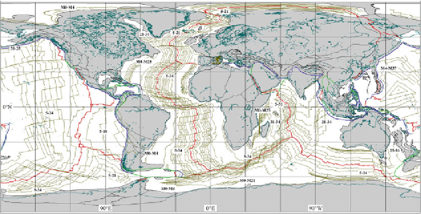
Fig. 5.16 Global isochron chart of Royer et al. ( 1992 ). Labels are anomaly names of the corresponding isochrons.
Modern plate boundaries and Mesozoic-Cenozoic tectonic elements are also displayed

that only include isochrons at stage boundaries.
For instance, the first digital global compilation
of isochrons from the World's oceans (Royer
et al. 1992 ), which led to the well-known age
map of the sea floor of Müller et al. ( 1997 ),
included isochrons for only 14 anomalies: 5, 6,
13, 18, 21, 25, 31, 34, M0, M4, M10, M16,
M21, and M25. In that model, the ages of these
anomalies were identified as global synchronous
stage boundaries (see Sect. 2.7 ) , at which sharp
changes of the stage poles occurred. We shall
come back to this point in the next chapter.
Figure 5.16 shows the original isochron chart of
Royer et al. ( 1992 ), combined with the global
compilation of tectonic elements of Schettino and
Scotese ( 2005 ), some additional isochrons for
the western Mediterranean (Schettino and Turco
2006 ), and a couple of synthetic (i.e., theoretical)
isochrons for the Canada Basin area (based on
the model of Rowley and Lottes 1988 ). This map
illustrates the major tectonic features associated
with the evolution of the oceanic basins since
the middle Jurassic, including ridge jumps, ridge
extinctions, changes of the stage pole, subduction
of spreading centers, and the location where the
Pacific plate formed as a small oceanic plate
bounded by three ridges. However, the isochrons

also represent the geometrical expression of a
statistical procedure that allows to determine fi-
nite reconstruction poles starting from locations
of identified magnetic anomalies and fracture
zones.
Now we are going to describe this proce-
dure in detail. The starting point for the con-
struction of isochrons is represented by a com-
bination of ship track magnetic anomalies and
fracture zones. To build a reliable map, it is
necessary to have at least two magnetic profiles
crossing each spreading ridge segment, and a
digitized data set of fracture zones. An exam-
ple of variable data coverage is illustrated in
Fig. 5.17 .
The second step consists into the analysis of
the magnetic profiles, according to the proce-
dure illustrated in the previous section. This step
provides, for each profile, a sequence of apparent
spreading velocities, which can be converted into
a series of locations along the projection line.
These locations correspond to the starting offset
of each block in the magnetization model and
are called crossing points or simply crossings .
They specify where a certain anomaly can be
found. Therefore, the set of all crossings corre-
sponding to a given anomaly represents the basic