Geology Reference
In-Depth Information
field vector during the corresponding chrons. In
plate kinematics, the magnetization direction of
a prism cannot be chosen as coincident with the
present day reference field
F
, not even when the
data ages encompass the last 2-3 Myrs. In fact,
assuming that the rock magnetization is entirely
of NRM type, even in the case of rocks that
formed during the last polarity chron, the average
magnetization direction would be aligned with
the
time
-
averaged geomagnetic field
for the last
0.78 Myrs, which is a GAD field. Therefore,
in this instance the paleomagnetic direction in
(
5.49
)and(
5.50
) would be
I
D
90
ı
,
D
D
0
ı
and
not
that of the local IGRF field (i.e.,
I
0
and
D
0
).
These parameters can also be used for rocks of
Pliocene - Pleistocene age, but in general older
crust requires a different approach. In the next
chapter, we shall see that for a tectonic plate that
has been moving around the globe, the NRM
directions of its rocks of various ages can be de-
scribed by a temporal sequence of paleomagnetic
fields whose dipole axes migrate in a regular fash-
ion away from the present day Earth's spin axis
according to an age progression. This
apparent
polar wandering
, which is a consequence of plate
motions, must be taken into account in plate kine-
matics modelling, because it determines a corre-
sponding change of paleomagnetic directions in
so far as we move away from a spreading centre.
Let (
p
1
,
p
2
, :::,
p
n
) be a sequence of paleopole
positions for one of the two conjugate plates
about a spreading ridge. This sequence furnishes
the apparent orientation of the spin axis (i.e.,
the apparent location of the geographic North
Pole) during each chron in the time scale, as
seen from the reference frame of this plate. In
the next chapter, we shall study in detail these
apparent polar wander paths
(APW Paths). For
the moment, it is sufficient to say that we can
easily compute the paleomagnetic inclination and
declination (
I
k
,
D
k
) of the NRM vector at any
point along the projection line starting from these
paleopoles. A similar procedure can be used to
determine the inclination and declination (
I
0
k
,
D
0
k
)
for any point on the tract of projection line placed
on the opposite side of the spreading ridge. To
this purpose, it could be necessary to have a
sequence of paleopoles (
p
0
1
,
p
0
2
, :::,
p
0
n
)alsofor
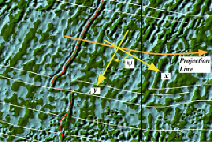
Fig. 5.10
Example of determination of the profile obliq-
uity angle §
§ that is greater than 90
ı
even in the case of a
projection line oriented as the fracture zones,.
Once the data have been projected, it is nec-
essary to assign the position of the
origin
along
the magnetic profile, which will be the point
with offset zero in age-distance plots. This point
should be placed tentatively along the spreading
ridge (or the extinct ridge) as seen on gravity
anomaly maps. However, it will be adjusted later
to match the observed central anomaly. In order
to start a forward modelling procedure, we must
assume an initial spreading velocity
v
,which
will be used to build the initial configuration of
the magnetized prisms according to a selected
Very often, the prisms are draped on bathymetry,
with constant height
H
equal to the assumed
magnetized layer thickness, but it is also possible
to build models that are based on estimates of
the real depth to the basement (excluding the
sedimentary layer).
For each chron in the time scale, a polygon
that approximates the cross-section of the crustal
block that formed during this time interval is
built, with horizontal width
w
k
proportional to the
chron duration:
1
2
v
T
k
w
k
D
(5.60)
where
v
is the default full spreading rate and
T
k
is the duration (in Myrs) of the
k
-th chron.
The polygons are assumed to have uniform mag-
netization directed as the average paleomagnetic