Geology Reference
In-Depth Information
having primarily frequencies of 24, 12, 8, and 6 h
and amplitudes of only a few tens nT. However,
we have seen that the external contribution to
the geomagnetic field can reach 1,000 nT during
magnetic storms. Finally, the third important con-
tribution to the total magnetic field is represented
by an “anomalous” field
F
D
F
(
r
,
t
) (intended
as perturbation of the main core field) associated
with the remnant and induced magnetizations of
crustal rocks. This field can be considered as a
time independent field when the main component
of magnetization is the remnant magnetization,
a condition which is generally met by oceanic
magnetic field vector that is observed at the
Earth's surface can be written as follows:
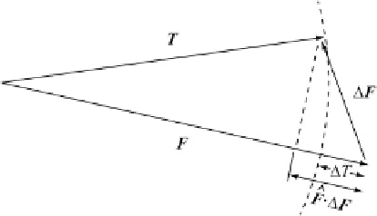
Fig. 5.1
Relationship between main (
core
)field
F
, ob-
served field
T
, and anomalous field
F
in the definition
of magnetic anomalies
observed data. Now we want to give a physical
significance to the expression (
5.2
). To this pur-
pose, we note that the field
F
in (
5.1
) can be
considered as a small perturbation to the main
reference field, caused by the magnetization of
crustal rocks. In fact, ignoring the external con-
tribution, the average magnitude of the observed
field is
45,000 nT, whereas crustal field mag-
nitudes in the oceans generally do not exceed
500 nT.
Following Blakely (
1996
), we also observe
that the total field anomaly
T
defined in (
5.2
)
is not equivalent to the magnitude of the anoma-
lous field,
F
, because
T
Dj
F
C
F
jj
F
j
¤
F
, as illustrated in Fig.
5.1
.However,for
F
<<
j
F
j
we can write:
T .r;t/
D
F .r;t/
C
S .r;t/
C
F .r/ (5.1)
A
total field magnetic anomaly
is calculated
from
scalar
field measurements by subtracting
the reference core field, usually an IGRF, and
eventually applying a diurnal correction, which
removes those components of the measured field
associated with solar and ionospheric activity.
Let
T
D
T
(
r
,
t
) be the observed magnitude of
total field at location
r
and time
t
, which can be
obtained by a scalar magnetometer survey. Let
F
D
F
(
r
,
t
) be the IGRF field at the same point
and time. Finally, let us assume that an estimate
of the external contribution to the magnitude of
the observed field, that is a
diurnal correction
S
D
S
(
r
,
t
), is available. Then the total field
anomaly is defined as:
T
Dj
F
C
F
jj
F
j
Š
p
F
F
C
2F
F
j
F
j
D
F
r
1
C
2
F
F
F
F
F
Š
Š
F
1
C
F
F
F
F
T .r;t/
D
T.r;t/
F.r;t/
S .r;t/
(5.2)
F
D
F
F
F
F
F
D
F
F
(5.3)
In the next section, we shall see that an esti-
mation of the external components in Eq. (
5.2
)
can be performed using nearby magnetic obser-
vatory data and/or a special design of the survey
tracks. Unfortunately, most oceanic surveys are
performed far away from magnetic observatories,
and the ship-track design generally must satisfy
the requirements of other kinds of geophysi-
cal measurement. Therefore, the calculation of
marine magnetic anomalies is often performed by
simple subtraction of the reference field from the
Therefore, a total field anomaly
T
approximately coincides with the
projection
of the anomalous field
F
onto the reference
field axis. In other words,
T
approximates
the component of the field generated by the
crustal sources in the direction of the regional
field. Typical total field oceanic anomalies range
from a few nT to thousands of nT, with an rms
value of 200-300 nT. Therefore, the condition
j
F
j
>>
F
is usually met. Note that in general