Geology Reference
In-Depth Information
LJ
LJ
LJ
LJ
rDa
D
sin ™
X
n;m
1
r sin ™
@V
@
¥
1
@Y
n
@
¥
v
n
(4.114)
Therefore,
v
n
@Y
n
r
s
V
j
rDa
D
X
n;m
1
sin ™
@Y
n
@™
™
C
@
¥
¥
D
X
n;m
v
n
r
s
Y
n
j
rDa
(4.115)
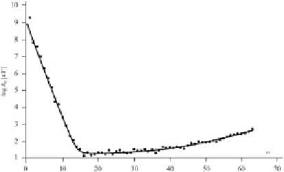
Fig. 4.26
Power spectrum of geomagnetic field accord-
ing to the field model of Cain et al. (
1989
)
Substituting (
4.112
)and(
4.115
)into(
4.106
)
gives:
8 a
2
0
X
n;m;s;r
2
0
ǝ
B
2
Ǜ
S.a/
D
1
1
R
n
D
.n
C
1/
Cn
X
.n
C
1/.s
C
1/
v
n
v
s
2
n
j
v
n
j
m
D
I
1
8 a
2
0
h
g
n
2
C
h
n
2
i
(4.119)
X
n
Y
n
Y
s
dS
C
D
.n
C
1/
S.a/
mD0
v
n
v
s
I
S.a/
X
n;m;s;r
r
Y
n
r
Y
s
dS
By analogy with time domain spectral analy-
sis, a plot of
R
n
as a function of
n
can be called
the
power spectrum
(Lowes
1974
). Figure
4.26
shows the power spectrum for the field model
of Cain et al. (
1989
). We note that the spectrum
breaks into two parts, with a transitional region
from
n
D
13 to
n
D
16. An obvious interpretation
of this result is that the two spectra are expres-
sions of distinct sources. In fact, there exists
very strong evidence that the terms from
n
D
1
to
n
D
13 are representative of the core field,
whereas the crustal contribution would be limited
to the terms with
n
>13. However, this separation
of core and crustal terms is not perfect, because
large-scale features of the crustal field are also
contained in the terms from
n
D
1to
n
D
13, just
as short wavelength features of the core field are
included in the
n
>13 series.
The
International Geomagnetic Reference
Field
(IGRF) is a geomagnetic field model
representative of core sources, produced and
maintained by a team of modelers under the
auspices of the
International Association of
Geomagnetism and Aeronomy
(IAGA). It is
based on a least squares parametric regression
of observed data by a truncated version of the
spherical harmonic expansion (
4.93
). The highest
(4.116)
The two integrals at the right-hand side of
(
4.116
) can be converted to integrals over the unit
sphere by multiplying both terms by
a
2
. Then,
applying the orthogonality conditions (
4.96
)and
(
4.110
) we obtain:
X
.n
C
1/
2
2n
C
1
j
v
n
j
2
0
ǝ
B
2
Ǜ
S.a/
D
1
1
2
0
2
n;m
2
0
X
n;m
1
n.n
C
1/
2n
C
1
j
v
n
j
2
C
(4.117)
Finally,
ǝ
B
2
Ǜ
S.a/
D
X
n;m
.n
C
1/
j
v
n
j
2
(4.118)
This is an important result, which establishes
how the average squared magnitude of the geo-
magnetic field over the reference surface depends
from the various harmonics and wavelengths. Let
us introduce the quantity: