Geology Reference
In-Depth Information
core (we shall face the dynamics of fluids in
differential equations is necessary to determine
the evolution of the Earth's magnetic field. The
Earth's magnetic field model of Glatzmaier
and Roberts (
1995
) is precisely the result of
a numerical solution to the induction equation
and related fluid dynamics and electromagnetic
equations. We shall not investigate further this
rather complex subject. However, in the next
section, we are going to discuss a conceptual
(analog) model for the generation of the
geomagnetic field, starting from Faraday's law.
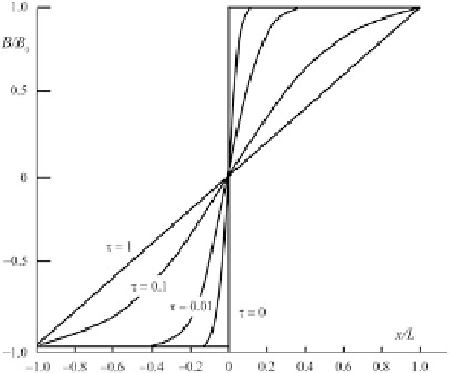
Fig. 4.2
Distribution of the magnetic field for different
values of the non-dimensional time
£
ǜ
t
/
L
2
predicted
by (
4.18
). It is apparent the progressive smoothing of the
field with time
D
4.2
The Geodynamo
Let us consider first the electrostatic field
E
D
E
(
r
) generated by a system of electric charges
(Eq.
4.5
). This is a
conservative field
, such that
the work
W
done in moving a particle from a
point
P
1
to another point
P
2
does not depend
from the path between the two points. In this
case, a scalar function
V
D
V
(
r
) exists such
that:
and an arbitrary initial profile
B
(
x
,0)
D
f
(
x
), it
is possible to show that the field decays rapidly
to zero on a time scale given by £
D
.Inthe
case of the Earth, the geomagnetic field would
disappear within 10
5
years. Consequently, the
induction term
r
(
u
B
)in(
4.14
) is effective to
contrast the decay associated with diffusion. For
example, if we set the diffusion term in (
4.14
)to
zero, which is equivalent to assume a very high
conductivity of the fluid, then the magnetic field
lines would be “frozen” into the fluid and would
always be moving with it.
So far, we have considered the effect of con-
vective motions for the maintenance of a mag-
netic field within the outer core. Now we want
to briefly mention the action exerted to the fluid
back by the magnetic field. We know that a
Lorentz force is exerted on a moving charged par-
case of a fluid, which can be represented as a con-
Lorentz force per unit volume,
f
, will given by:
E
Dr
V
(4.21)
The function
V
is called
electrostatic potential
and its units are [V]. Then, the work per unit
charge will be given by:
Z
Z
P
2
W.P
1
;P
2
/
D
E .r/
dr
D
r
V
dr
P
1
Z
P
2
@V
@r
dr
D
V.P
1
/
V.P
2
/
D
P
1
(4.22)
Therefore, the integral of
E
along any closed
loop
f
D
¡.
v
B/
D
j
B
(4.20)
is zero:
I
This force must be incorporated into the
fluid dynamics equations describing the relation
between forces and accelerations in the liquid
E
dr
D
0
(4.23)