Geoscience Reference
In-Depth Information
2
X
n
t
c
n
x
ð
c
n
x
ð
E
¼
observed
Þ
predicted
Þ
(5)
m
¼
1
The model fit to the observations was optimised by adjusting the parameters
(
u
,
D
,
k
1
,
A
s
/
A
) strategically in order to minimise
E
. Note that lateral inflow (
q
) was
obtained directly from solute dilution calculations and was therefore not adjusted as
a fitting parameter. The parameter optimization was undertaken with a direct search
method, this being a SIMPLEX method of the Nelder-Mead variety (Lagarias et al.
1998
). The numerical solution was coded in FORTRAN and then compiled and
linked with the MATLAB mex libraries to create a dynamic linked library, which is
a callable function within MATLAB.
5 Results and Discussion
5.1 Pooled Analysis
The model was optimised to several tracer data sets from both the summer and
spring conditions to obtain stream transport parameters (
u
,
D
,
k
1
,
A
s
/
A
) over a range
of flow conditions (flows varied from 1 to 16 L/s in the experiments considered).
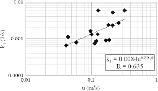
Figure
2
shows a plot of the transient storage exchange parameter (
k
1
) versus flow
velocity. We might expect that these parameters would correlate with each other; at
larger velocities the shear gradient across the boundary layer will be larger with
consequently larger mass transport. Admittedly the flow field in these small streams
is much more complicated than the simple shear flow for which this exchange
mechanism is envisaged and there is considerable scatter; however, we observe a
fairly strong correlation (
R
¼
0.635,
n
¼
16) when a power law model is fitted; we
Fig. 2 Plot of transfer coefficient (
k
1
) versus velocity (
u
) for all studied streams pooled from
summer and spring