Geoscience Reference
In-Depth Information
a
b
18
18
16
14
12
10
8
6
4
0.1
16
14
12
10
8
6
4
0.1
1.0
10.0
100.0
1.0
10.0
100.0
y
/
Δ
y
/
Δ
c
d
18
18
16
14
12
10
8
6
4
0.1
16
14
12
10
8
6
4
0.1
1.0
10.0
100.0
1.0
10.0
100.0
y
/
Δ
y
/
Δ
E1
E0
E2
E3
E1D
E2D
E3D
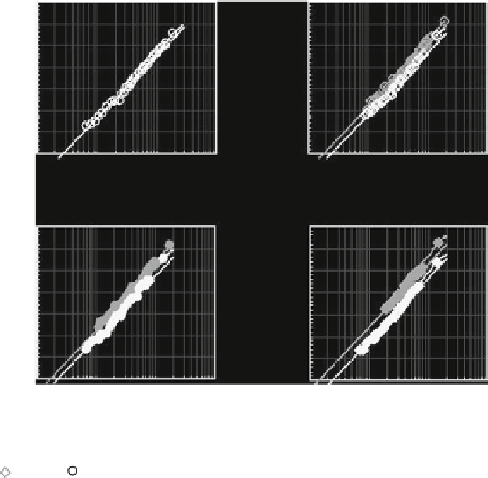
Fig. 18 Velocity profiles: (a) E0, (b) E1 and E1D, (c) E2 and E2D, and (d) E3 and E3D. Best fit
lines: mobile bed
; fixed bed
The hydrodynamical conditions are shown next. The time-averaged and ensem-
ble averaged longitudinal velocity profiles are shown in Fig.
18
. The ensemble
average is a result of four independent measurements per point. The solid lines
represent the log-wake law for rough beds:
þ
1
k
ln
y
k
s
2
P
k
sin
2
p
y
2
h
u
þ
¼
B
r
þ
(8)
where
u
+
¼
u
/
u
*
;
u
¼
the longitudinal time-averaged velocity;
y
¼
height above
some datum;
k
s
¼
scale of the roughness elements;
P ¼
Coles' parameter; k
¼
von
K´rm´nconstant(k
constant depending on roughness geometry.
The scale of the roughness elements was taken to be equal to the maxi-
mum amplitude in the bed texture series for the fixed bed tests. This method
was not applied in the mobile bed tests since it is not possible to distinguish
which grains are actually felt as roughness by the flow. In that case,
k
s
was
related to the thickness of the bed-load layer and taken to be the
d
90
of the bed-
load distribution.
¼
0.4); and
B
r
¼