Biology Reference
In-Depth Information
100
100
80
80
60
60
40
40
20
20
10
20
30
40
50
60
70
80
90
100
110
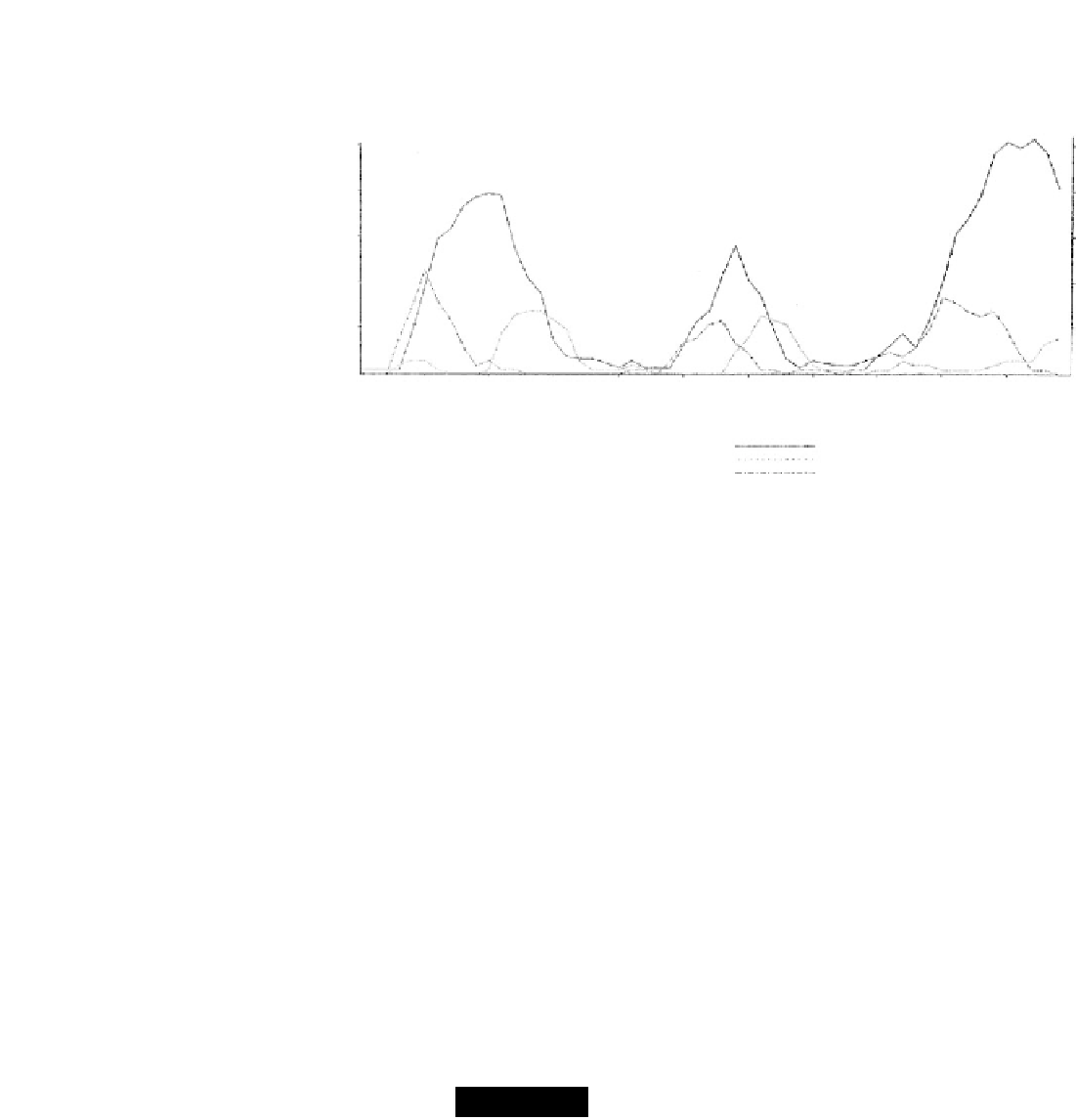
TIME IN DAYS
GRAPH III. Mechanism of oscillation at 25
C.
Legend: Population size
Deaths*
Births*
* If the actual number of deaths and births occurring on each day is plotted, the resulting curves are too irregular and too low to read
with ease. Accordingly, each number was doubled, and the curves smoothed by plotting the points as 3-point moving averages.
FIGURE 1-21.
Oscillations in the size of a water flea (Daphnia) population. (From Pratt, D. M. [1943]. Biological Bulletin 85, 116-140. Used
by permission.)
to offset the dependence r(t)
r(P(t)) to account for this time lag. In
nonmathematical terms, we say that the present value of r(t)is
determined by the population size at a specific time in the past. The
simplest way to model this is to postulate that r(t)
¼
¼
r(P(t
D)), where
>
D
0 is the measured delay. In the example above, D will be equal to
nine months—a baby's average gestational period. The logistic model
(1-12) can now be modified so:
P
ð
Þ
dP
dt
¼
P
t
D
a 1
ð
t
Þ:
(1-28)
K
Notice that this model preserves our fundamental hypothesis that
the rate of change in population size is proportional to the population
size.
E
XERCISE
1-13
List the limitations of the model given by Eq. (1-28).
The model from Eq. (1-28) is quite different mathematically from the
logistic model. To obtain an exact analytical solution for Eq. (1-28), we
need to know the values of the solution P(t) over the whole interval
[0,D]. In contrast, knowing the value of P(t) at just one point, say t
¼
0, is