Biology Reference
In-Depth Information
in similar output, and similar options are available in SPSS Trends
and SAS.
If the input time series for ARFILTER is x(t), the algorithm produces
an output series u(t) that represents the low-frequency component(s)
of the original data series. The filtering procedure uses a single
parameter
, the value of which is optimized so that the residuals,
defined by [x(t)
r
u(t)], are least-squares minimized, as described in
Chapter 8. The detrended residuals [x(t)
u(t)] then represent the
residual high-frequency component(s) that were filtered out by this
forward-backward autoregressive filtering process. It is important to
note that, depending on the situation, either u(t)or[x(t)
u(t)] may be
used in subsequent analysis: u(t) if the objective was to remove
excessive high-frequency noise from the original data series, and
[x(t)
u(t)] if the objective was to remove confounding, low-frequency
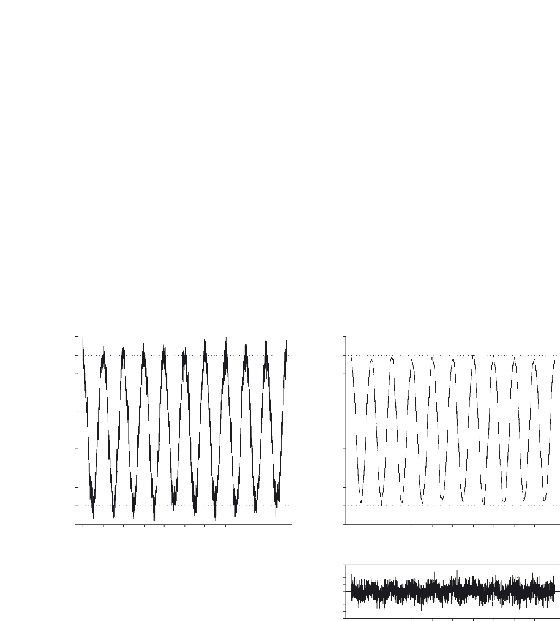
trending from the original data series. Figures 11-16 and 11-17 illustrate
the use of ARFIILTER with the noisy simulated data sets from
Figures 11-14 and 11-15. The time series u(t) and [x(t)
u(t)] are
presented to the right of the original time series x(t). An important
100
125
100
100
75
75
50
50
25
25
−
0
0
−
25
−
25
−
50
−
50
−
75
−
75
−
100
−
100
−
125
−
125
0
24
48
72
96 120 144 168 192 216
240
0
24
48
72
96 120 144 168 192 216
240
Time (hours)
Time (hours)
40
1
2
30
ARFILTER Analysis of
Noisy Stationary Cosine Wave
−
1
0
−
20
−
30
−
40
0
24
48
72
96 120 144 168 192 216
240
Time (hours)
FIGURE 11-16.
Example of ARFILTER applied to a noisy stationary cosine wave.