Biology Reference
In-Depth Information
The period is, therefore, larger than 24 hours. In this particular example,
the data also indicate that the phase shifts in a linear fashion, by about
2.6 hours per day—the slope of the line formed by the data points.
Observing a linear pattern with positive slope would correspond to a
constant period greater than 24 hours. In the laboratory project for this
chapter, we observe other functional dependencies.
2.5
2
1.5
1
0.5
0
−
0.5
−
1
−
1.5
−
2
−
2.5
0
2
4
6
8
10 12 14 16 18
20
A
Time
E
XERCISE
11-1
2.5
2
Describe the characteristics of a plot depicting the time of daily
acrophase for time series exhibiting a constant period of magnitude
smaller than 24 hours.
1.5
1
0.5
0
−
0.5
−
1
−
1.5
−
2
−
2.5
0
1
2
3
4
5
B
B. Using Simulated Data
Time
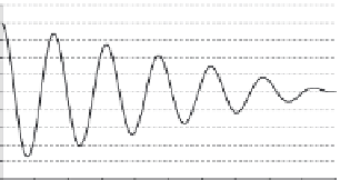
FIGURE 11-12.
A cosine-like rhythmic pattern with decreasing
amplitude (panel A) and shrinking period (panel B).
As discussed previously, many data analysis algorithms are first verified
on simulated data. The major point here is that for simulated data, the
answers we would normally want to find in a data set are already
known. So, the efficiency of any new data analysis method is generally
first tested on a simulated data set. When more than one algorithm is
available for a particular task, they can be compared on the basis of the
closeness of their generated answers to the actual simulation values. For
example, Figure 11-14 presents a graphical depiction of the fundamental
phenomenologically defining properties exhibited by rhythms of a
cosine wave that is mean and variance stationary, but does contain
additive noise. The data have:
1. A mean expression intensity of 0 y-axis units;
2. An oscillatory amplitude of 100 y-axis units;
3. A period of oscillation of 24 hours;
4. A phase reference point, in this case the time of acrophase, at
0 hours; and
5. Gaussian-distributed random noise added, such that the standard
deviation of the noise is 10 y-axis units.
The situation becomes more challenging when the data contain a trend
and the variance of the data changes with time. Figure 11-15 introduces
mean and variance nonstationarities on top of a rhythm similar to that
presented in Figure 11-14. The data set in Figure 11-15 represents a
cosine wave possessing mean and variance nonstationarities exhibiting:
1. A mean expression intensity that is time-dependent, such that at
time zero, the mean expression intensity is 1000 y-axis units,
but it decays in magnitude in exponential manner to a final