Biology Reference
In-Depth Information
E
XERCISE
10-2
Z
t
e
að
t
z
Þ
dz, then
dC
Þ
dt
¼a
ð
t
Prove that if C
ð
t
Þ¼
S
ð
z
Þ
C
ð
t
Þþ
S
ð
t
Þ:
1
Hint: Follow the outline below:
e
a
h
Z
t
þ
h
e
að
t
z
Þ
dz
1. Show that C
ð
t
þ
h
Þ¼
S
ð
z
Þ
:
Z
t
1
e
að
t
z
Þ
dz
e
a
h
2. Show that C
ð
t
þ
h
Þ
C
ð
t
Þ¼ð
1
Þ
S
ð
z
Þ
þ
e
a
h
Z
t
þ
h
1
e
að
t
z
Þ
dz
S
ð
z
Þ
:
Z
t
þ
h
t
e
a
h
e
a
h
h
3. Show that
C
ð
t
þ
h
Þ
C
ð
t
Þ
1
e
að
t
z
Þ
dz
¼
C
ð
t
Þþ
S
ð
z
Þ
:
h
h
4. Finally, to prove that
dC
Þ
dt
¼a
ð
t
t
C
ð
t
Þþ
S
ð
t
Þ
, use
Z
t
þ
h
e
a
h
1
h
1
e
að
t
z
Þ
dz
lim
h
S
ð
z
Þ
¼
S
ð
t
Þ
, and lim
h
¼a:
h
!
0
!
0
t
Equation (10-1) can be implemented as a model describing the rate
of change of hormone concentration in response to a specific pattern
of hormone delivery/secretion. In the following two examples, the
numerical simulations were performed with BERKELEY MADONNA.
Example 10-4
.........................
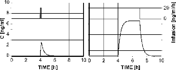
The plots in Figure 10-7 depict the simulated dynamics of a hormone in
the circulation providing it is released endogenously (secreted
internally) or administered exogenously (external delivery) as a bolus
(left panel) or in a nonvarying fashion (right panel). In both simulations,
the clearance constant is
3h
1
and the secretion (or infusion) rate is
20 ng/ml/h. The secretion is continuing for 10 minutes (left panel) or
180 minutes (right panel).
a ¼
FIGURE 10-7.
Approximation of the raise and decay of a hormone administered as a (short-term) 10-minute (left)
or (long-term) 3-hour constant infusion (right). The bottom line depicts the hormone concentration
evolution, while the top curve illustrates the pattern of hormone delivery.