Biology Reference
In-Depth Information
the same distribution. But
1
þ
2
is the number of heads
on both flips. The possibilities are HH, HT, TH, and TT, so the
probabilities that
1
þ
2
takes values 2, 1, and 0, respectively, are
P
ð
1
þ
2
¼
2
Þ¼
1
=
4, P
ð
1
þ
2
¼
1
Þ¼
1
=
2, and P
ð
1
þ
2
¼
0
Þ¼
1
=
4.
An important property of the normal distribution is that when we add
two independent random variables
x
and
that are normally
0.14
distributed, the sum
also has a normal distribution with mean
equal to the sum of the means and variance equal to the sum of the
variances of
x þ
0.12
0.10
0.08
, however,
will no longer result in normal distribution. We next consider several
other probability distributions that are derived from the normal
distribution and used for various statistical tests. We shall introduce
them briefly, without the cumbersome formulas for their densities.
Figure 4-2 shows the graphs of these densities for various choices of
parameters.
x
and
. Other operations performed on
x
and
0.06
0.04
0.02
A
0.00
0
2
4
6
8
10121416182022242628303234363840
0.50
0.40
0.30
2
) distribution. This type of distribution arises when we
consider squares of random variables with standard normal distribution.
More specifically, if
Chi-square (
w
0.20
0.10
is a random variable with a standard normal
distribution, it may sometimes be necessary to consider
x
B
0.00
2
. Because
−
6
−
5
−
4
−
3
−
2
−
1
0
1
2
3
4
5
6
¼ x
x
is a random variable, so is
, but the density function of
cannot be
0.90
0.80
normal because the new random variable
takes only positive values.
0.70
2
distribution with one degree of freedom.Ifwe
consider several independent random variables
2
has a
We say that
¼ x
w
0.60
0.50
x
1
; x
2
;
...
; x
N
, all of
which have standard normal distributions, then we say the sum of the
squares of these random variables, namely
0.40
0.30
0.20
2
1
2
2
2
N
, has a
¼ x
þ x
þ
...
þ x
0.10
C
2
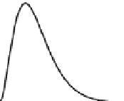
distribution with N degrees of freedom. Figure 4-2-(A) presents the
density function of a
0.00
w
0
1
2
3
4
5
6
2
distribution with N
w
¼
7 and N
¼
21 degrees of
FIGURE 4-2.
w
freedom, respectively.
2
, t- and F-distributions with varying parameters.
Panel A:
2
distribution with 7 (black) and
21 (gray) degrees of freedom; panel B:
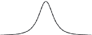
t-distribution probability density with 2 (black)
and 23 (gray) degrees of freedom; panel C:
F-distribution with 3, 40 (black) and 23, 8 (gray)
degrees of freedom.
w
t-(Student) distribution. This distribution arises when we need to consider
specific ratios of random variables. In particular, if
x
is a random
variable with a standard normal distribution and
is another random
2
distribution with N degrees of freedom, then their
variable with a
w
p
will be a new random variable. This new random variable
is said to have a t-distribution (or Student distribution) with N degrees
of freedom. The graphs of the probability density for t-distribution
with N
z ¼ x=
ratio
¼
2 and N
¼
23 degrees of freedom are shown in
Figure 4-2(B).
F-(Fisher) distribution: This distribution also arises when ratios of random
variables are considered, but this time it is the ratio of two random
variables with
2
distributions. More specifically, if
w
x
is a random
2
distribution with M degrees of freedom and
variable with a
w
is
2
distribution with N degrees of
another random variable with a
w
z ¼ x
freedom, then their ratio
will be a new random variable said to
have an F-distribution (or Fisher distribution) with M, N degrees of freedom.
/