Environmental Engineering Reference
In-Depth Information
4.3.3 M
eaSureMent
of
f
Low
Flows are typically measured by essentially computing an average velocity, which, when multiplied
by the cross-sectional area, is the low at that particular time and location. The average velocity for the
cross section can be computed using an area-weighted average. That is, the average velocity can be
computed by subdividing the cross section into many areas, each small enough that the velocity in that
piece could be assumed constant (see Figure 4.8). The velocity for each piece would be determined,
which, when multiplied by the area, yields a low. The total low would then be the sum of the indi-
vidual lows (
U
*
A
, where
U
is the velocity and
A
is the area), or the average velocity (
U
) determined
by the total low divided by the total area.
1
∫
(
)
U
=
A
u yz dApp
A
,
(4.1)
One practical question then is: how many lateral and vertical subdivisions are required to accu-
rately determine the low?
Stream gauging has a long history in the United States (see USGS 1995, 2000). The USGS is the
agency primarily responsible for gauging low in the United States and it maintains over 7000 gauging
stations, constituting over 90% of the nation's gages (Hirsch and Costa 2004). Other agencies respon-
sible for low and/or water surface elevations measurements include the U.S. Army Corps of Engineers
(the Corps), the National Weather Service, the Bureau of Reclamation, and other federal and state agen-
cies. It is also not uncommon for industries to gage receiving waters as they impact permit compliance.
The traditional method used by the USGS for measuring the low at each station is to subdivide
the cross section into a minimum of 20 lateral sections and then determine the average velocity for
each section; the total low is the sum of the sectional lows. The USGS guideline for the number
of points required to determine the vertically averaged velocity is based on an assumed velocity
distribution. The assumptions include that the river low is predominantly one-dimensional, the low
is constant with time (steady low over the measurement period), and the river is wide, so that the
velocity proiles in the river cross section are not affected by the presence of banks. The velocity
Distance
0.2 0.3 0.4 0.5 0.6
0.7 0.8
0.8 1.0
1.0 1.0 1.0 0.9 0.8
0.7
0.6 0.4
0.2
0.2
0.3
0.4 0.5 0.6
0.6
0.8 0.8
1.0 1.0 1.0 1.0
0.8
0.8
0.7
0.4
0.3
0.1
0.1
0.3
0.3 0.3
0.3 0.3 0.3
0.4
0.5 0.5
0.6
0.7 0.7
0.9 0.9 0.9 0.9
0.8
0.7
0.6
0.3
0.2
0.7 0.7 0.7 0.7
0.4
0.4 0.4
0.5 0.5 0.5
0.6
0.5
0.2
0.2
0.4 0.4 0.4
0.5 0.5 0.5 0.5 0.5
0.4
0.3
0.2 0.2
0.3 0.3 0.3
0.4 0.4 0.4 0.4 0.4
0.2 0.2 0.2 0.2 0.2 0.2
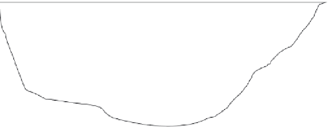
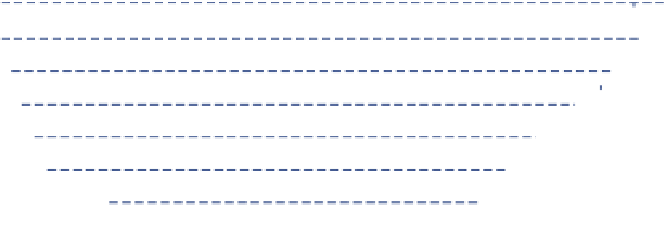
FIGURE 4.8
Flow characterization in a river. (From Winkler, M.F., Acoustic Doppler current proilers
broadband band and narrowband technology explained, USACE Engineering Research and Development
Center, Vicksburg, MS, 2006.)


Search WWH ::

Custom Search